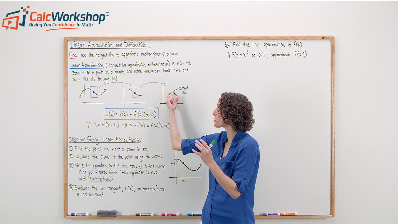
This lesson is about using the tangent line to approximate another point on our curve.

Jenn, Founder Calcworkshop®, 15+ Years Experience (Licensed & Certified Teacher)
What Is Linear Approximation
The idea behind local linear approximation, also called tangent line approximation or Linearization, is that we will zoom in on a point on the graph and notice that the graph now looks very similar to a line.
This means that we can use the tangent line, which rests in closeness to the curve around a point, to approximate other values along the curve as long as we stay near the particular point.
Consequently, the equation of the tangent line, L(x), of a function, f(x), at x = a is written:
But in all honesty, this is nothing more than the equation of the tangent line we used in our previous lesson:
Simply put, linear approximation uses the fact that every curve will always look like a line if we zoom in small enough!
And it’s this fantastic fact that enables us to approximate another point on the curve that is close to our zoomed-in point.
How To Do Linear Approximation
- Find the point we want to zoom in on.
- Calculate the slope at that point using derivatives.
- Write the equation of the tangent line using point-slope form.
- Evaluate our tangent line to estimate another nearby point.
Example – Polynomial (Given An Initial Value)
Alright, so let’s put everything together and look at an example where we will use the equation of the tangent line to approximate a particular point on a curve.
Find the linearization of the function
- Step 1: Find the point by substituting into the function to find f(a).
- Step 2: Find the derivative f'(x).
- Step 3: Substitute into the derivative to find f'(a).
- Step 4: Write the equation of the tangent line using the point and slope found in steps (1) and (3).
- Step 5: Substitute x = 0.9 into the equation of tangent line found in step (4) and solve for y.
That’s it!
I want to draw your attention to the fact that if we merely substituted 0.9 directly into our function, we would arrive at the value of 2.43. Using our new method, we calculated the value to be 2.4.
Isn’t it amazing to see how accurate the equation of the tangent line is in approximating a curve near the point of tangency?
Therefore, as long as we say near our given point, our linear approximation will be very accurate. So, make sure you don’t stray too far from the point, as Paul’s Online Notes nicely states.
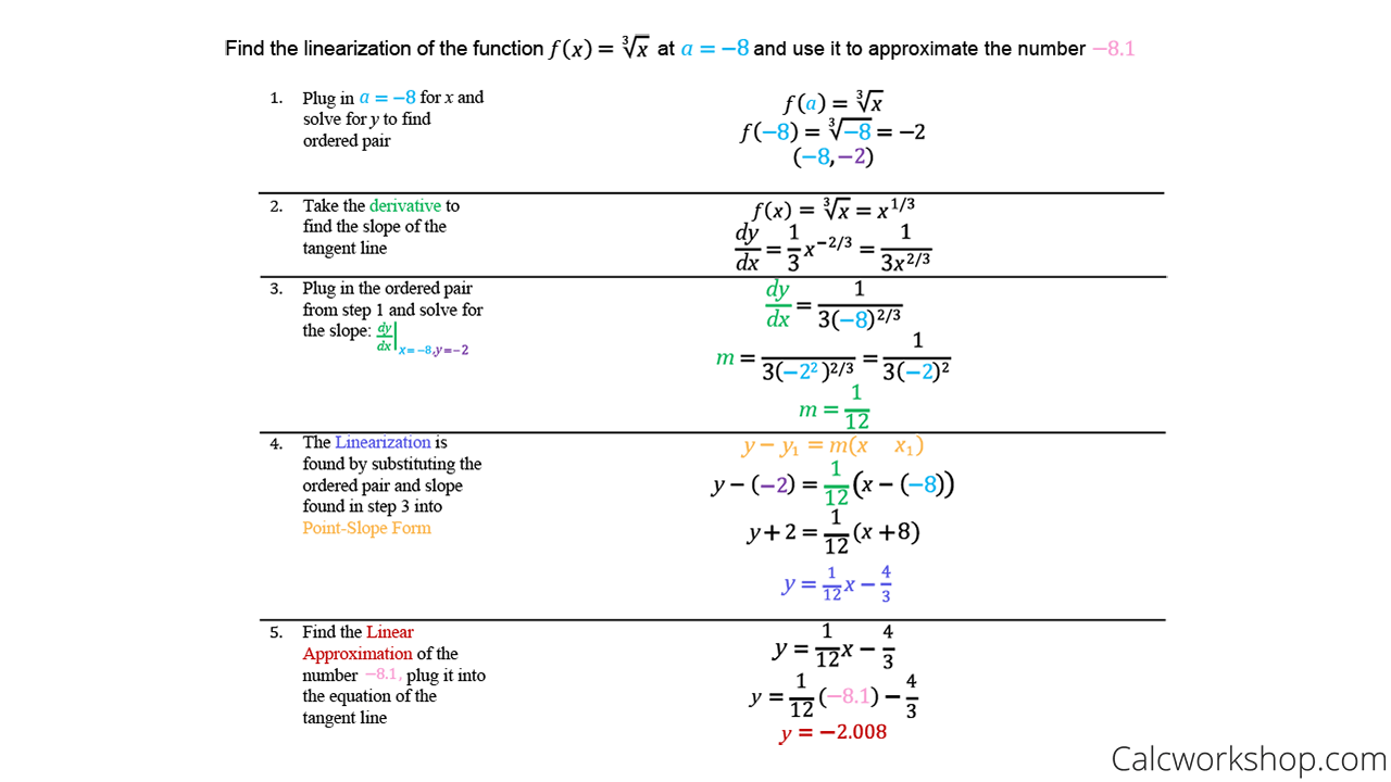
Example – Cube Root (Given An Initial Value)
Let’s now find f(-8.1) given

Linear Approximation Example
Nothing to it!
But the fun doesn’t stop here!
Did you know that the idea of differentials is based on the concept of linear approximation?
In fact, when we are asked to use differentials to estimate a given number, such as the square root or exponential, we are, in essence, being asked to use linearization to approximate the value.
In other words, with the help of tangent lines and a bit of calculus, we will become human calculators!
Example – Square Root
Let’s take a look at how we can use this method to approximate
- Step 1: Find a suitable function and center.
- Step 2: Find the point by substituting x = 49 into
- Step 3: Find the derivative f'(x).
- Step 4: Substitute x = 49 into the derivative f'(x).
- Step 5: Write the equation of the tangent line using the point and slope found in steps (2) and (4).
- Step 6: Substitute x = 50 into the equation of tangent line found in step (5) and solve for y.
Ask yourself, what is
Well,
Now, determine the type of function we are dealing with:
And guess what? If you plug
WOW! Aren’t we clever!
And finding the differential for exponential functions follows almost the same process as seen for the linear approximation of square roots.
Example – Exponential Function
Suppose we want to find the linearization for
- Step 1: Find a suitable function and center.
- Step 2: Find the point by substituting it into
- Step 3: Find the derivative f'(x).
- Step 4: Substitute into the derivative f'(x).
- Step 5: Write the equation of the tangent line using the point and slope found in steps (2) and (4).
- Step 6: Substitute x = 0.017 into the equation of tangent line found in step (5) and solve for y.
What is 0.017 close to?
0.017 is close to 0. Therefore, let’s choose x = 0 to be our center.
What is our function?
Summary
Isn’t it enthralling to know that you just did the same calculations as your calculator!
Gosh, we’re so talented!
So, together we will look at the overall process and idea behind linear approximation (i.e., linearization) and differentials.
Let’s get jump right in!
Video Tutorial w/ Full Lesson & Detailed Examples (Video)

Boost Your Calculus Scores with Step-by-Step Instruction
Jenn’s Calculus Program is your pathway to confidence. Each lesson tackles problems step-by-step, ensuring you understand every concept.
No more knowledge gaps – Jenn’s instruction bridges the missing pieces, so you’re always in stride with your class.
Calculus won’t block your academic or professional goals. Lay a solid foundation, one lesson at a time.
Your path to calculus success is just one click away.
Get access to all the courses and over 450 HD videos with your subscription
Monthly and Yearly Plans Available
Still wondering if CalcWorkshop is right for you?
Take a Tour and find out how a membership can take the struggle out of learning math.