Extrema Of Multivariable Functions
Explained w/ Step-by-Step Examples!

What do the words “open” and “closed” mean to you?

A place of business is either open or closed for customers.

There are open-ended or closed-ended question types.

And in object-oriented software development, there is something called the open-closed principle.

But the words open and closed also refer to how we go about finding absolute extrema and relative extrema.

Let’s take a closer look.

What Is Extrema

Single Variable

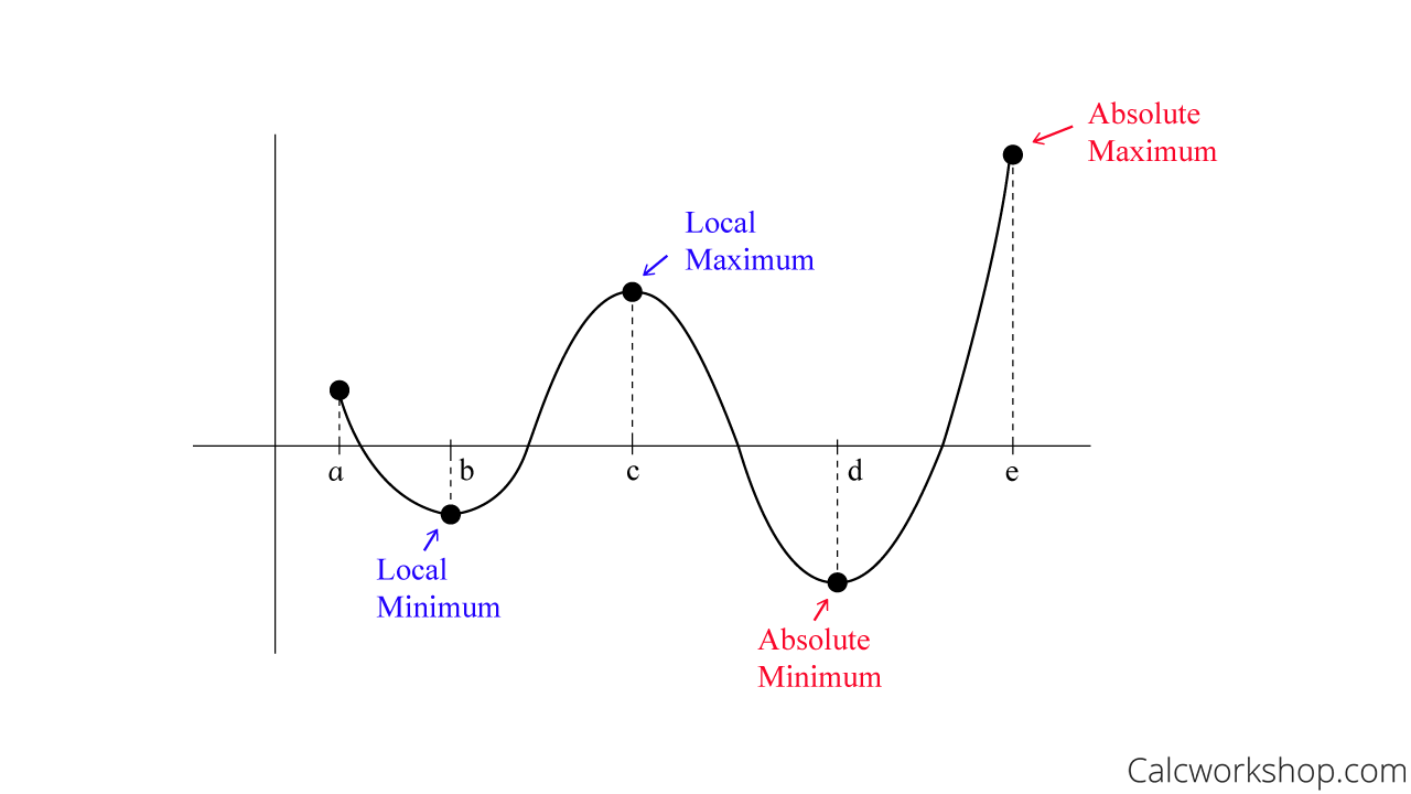
For functions of one variable, a continuous, differentiable function \(y = f\left( x \right)\) defined on a closed, bounded interval \(\left[ {a,b} \right]\) has an absolute (global) maximum and minimum occurring at a critical point in the open interval or at an endpoint.

The absolute extrema represent the highest and lowest points on a curve, whereas the term relative (local) extrema refer to any high and low point within the interval.

Multivariable

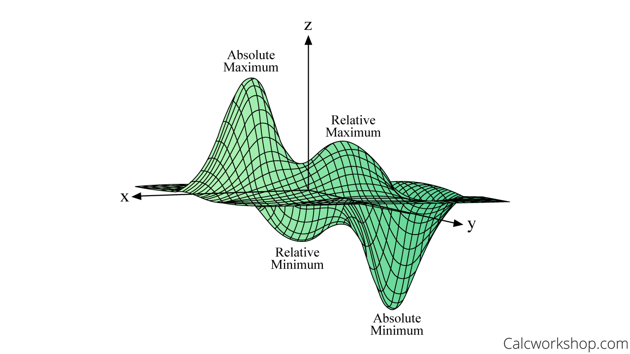
But what about functions of several variables?

Well, if \(f\) is a continuous, differentiable function, and \(S\) is a closed, bounded region, then \(f\) has both an absolute maximum and absolute minimum on \(S\).

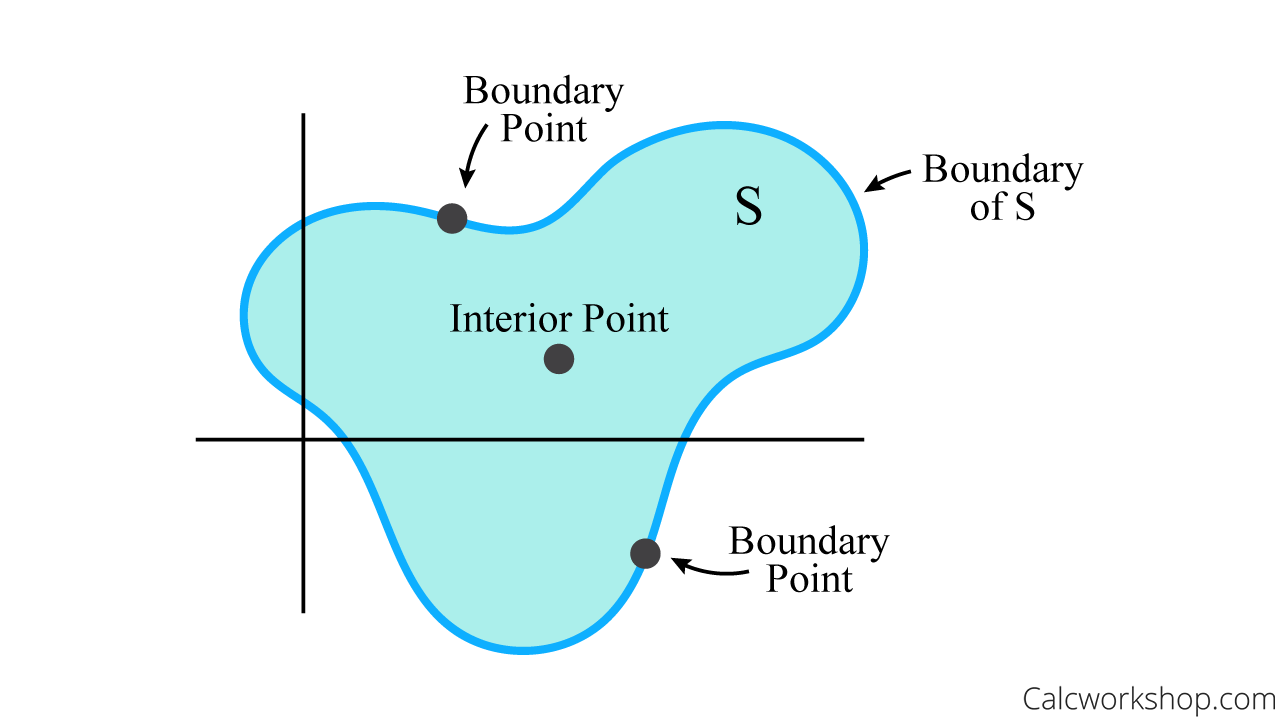
The difference between single and multivariable is that we are no longer dealing with an interval [a,b], but a region \(S\). Therefore, our analysis must include all critical points found in the interior of the region (interior points) and boundary points as well.

How To Find Global Extrema — Multivariable

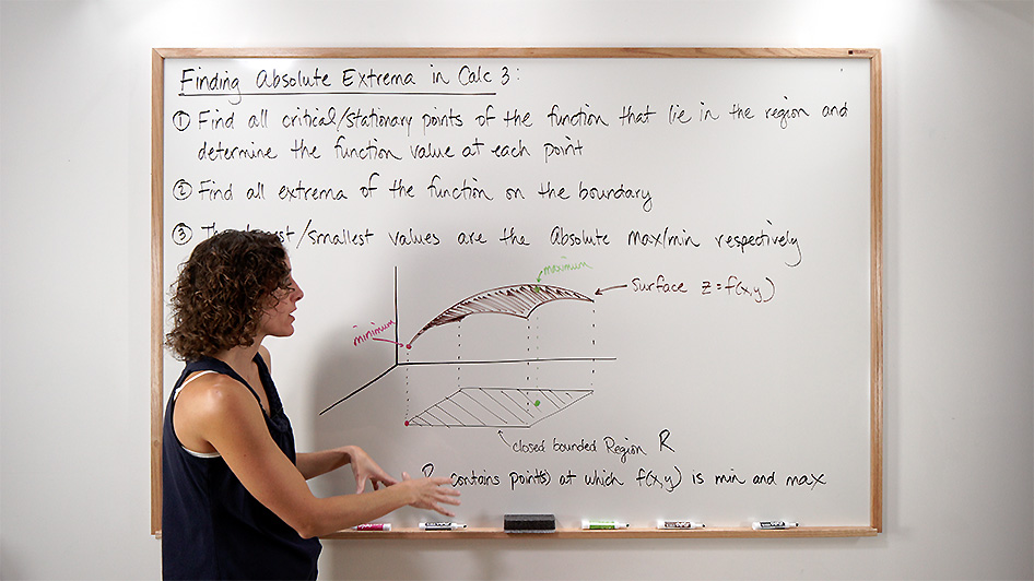
Thankfully, finding absolute extrema for functions of several variables is similar to those techniques we used in single variable calculus.

1. Identify critical points (stationary points) for the given function by setting the first order partial derivatives equal to zero and solving.
2. Then we will take our boundary and find new functions that could restrict or possibly yield a maximum and minimum value.
3. Lastly, we will substitute all critical points and boundary points into the original function, to determine the biggest and smallest values.

Example

Let’s work through an example to see these steps in action.

Determine the absolute maximum and minimum values for \(f\left( {x,y} \right) = {x^2} – {y^2} + 4\) on the disk \(S\), defined as \(S = \left\{ {\left( {x,y} \right):{x^2} + {y^2} \le 1} \right\}\).

So, first we will find the gradient vector \(\nabla f = \left\langle {{f_x},{f_y}} \right\rangle \) by calculating the first partial derivatives.

\begin{equation}
f_{x}=2 x \text { and } f_{y}=-2 y
\end{equation}

Next, we will set each partial derivative equal to zero to solve for any stationary points.

\begin{equation}
\begin{array}{cc}
f_{x}=0 & f_{y}=0 \\
2 x=0 & -2 y=0 \\
x=0 & y=0
\end{array}
\end{equation}

So, our critical point is \(\left( {0,0,f\left( {0,0} \right)} \right)\) or simply \(\left( {0,0,0} \right)\).

Now, we must turn our attention to the boundary \(S\) by substituting our boundary curve into our surface and simplifying.

If the boundary is \({x^2} + {y^2} = 1\) we can rewrite as \({x^2} = 1 – {y^2}\).

Thus, if \(z = f\left( {x,y} \right) = {x^2} – {y^2} + 4\) and \({x^2} = 1 – {y^2}\), then

\begin{equation}
\begin{aligned}
&z=\left(1-y^{2}\right)-y^{2}+4 \\
&z=3-2 y^{2}
\end{aligned}
\end{equation}

Notice that we now have an equation consisting of just a single variable. And how do we find a critical point of such an equation?

We take the derivative and set it equal to zero, just like we did in calculus 1!

\begin{equation}
\begin{aligned}
&\frac{d z}{d y}=-4 y \\
&-4 y=0 \\
&y=0
\end{aligned}
\end{equation}

Thus, if \({x^2} = 1 – {y^2}\) and \(y = 0\) then \(x = 1, – 1\).

And if \(z = f\left( {x,y} \right) = {x^2} – {y^2} + 4\), and \(y = 0\), or \(x = 1, – 1\), then \(z = 5, – 5\).

Therefore, we have two boundary points at \(\left( {1,0,5} \right)\) and \(\left( { – 1,0,5} \right)\).

But now, we need to solve our boundary curve for the other variable and see if there are any additional points we need to consider.

So, if \(z = f\left( {x,y} \right) = {x^2} – {y^2} + 4\) and \({y^2} = 1 – {x^2}\), then

\begin{equation}
\begin{aligned}
&z=x^{2}-\left(1-x^{2}\right)+4 \\
&z=3
\end{aligned}
\end{equation}

This indicates that \(x = 0\).

And if \({y^2} = 1 – {x^2}\) when \(x = 0\) then \(y = 1, – 1\).

Therefore, we have two more boundary points:

Now, all we have left to do is to analyze our five boundary points by utilizing our Second Partials Derivative Test for our critical point and then determining which point yields the biggest and smallest z-value.

\begin{equation}
\text { Absolute Maximum: }(1,0,5) \text { and }(-1,0,5)
\end{equation}
\begin{equation}
\text { Absolute Minimum: }(0,1,3) \text { and }(0,-1,3)
\end{equation}
\begin{equation}
\text { Saddle Point: }(0,0,0)
\end{equation}

This may seem challenging at first, but after walking through several examples in our video lesson where we will identify global maxima and minima, local minimum and maximum, and saddle points for multivariable functions, I’m confident you’ll get the hang of things.

So, together we are going to understand absolute extrema for functions of several variables and test both critical points and boundary points to identify global and local extrema.

Let’s get jump right in!

Video Tutorial w/ Full Lesson & Detailed Examples (Video)

Get access to all the courses and over 450 HD videos with your subscription

Monthly and Yearly Plans Available

Get My Subscription Now

Still wondering if CalcWorkshop is right for you?
Take a Tour and find out how a membership can take the struggle out of learning math.