Functions Of Several Variables (Introduction w/ Step-by-Step Examples!)

Did you know that many mathematical models involve functions of several variables?

Jenn (B.S., M.Ed.) of Calcworkshop® teaching functions of several variables

Jenn, Founder Calcworkshop^®, 15+ Years Experience (Licensed & Certified Teacher)

It’s true.

For example…

The ability to represent points on the surface of the earth.
Finding the work done by a force acting on an object.
Calculating the profit made from selling various items.
Or even finding the volume of a rectangular solid (i.e., V=lwh) all involve functions of two or more variables.

Domain And Range Of Multivariable Functions

So, a function $f$ of two variables is a rule that assigns to each ordered pair of real numbers $(x, y)$ in a set $D$ a unique real number denoted $f (x, y)$ . The set $D$ is the domain of $f$ and its range is the set of values that $f$ takes on, such that ${f (x, y) : (x, y) \in D}$ .

And for convenience we say $z = f (x, y)$ , just like we let $y = f (x)$ for functions of single variable. Thus, creating an explicit equation where $x$ and $y$ are independent variables and $z$ is the dependent variable.

But don’t worry.

Functions of several variables are just like functions of single variables.

Example #1 – Evaluate

For instance, suppose $f (x, y) = x + y^{2}$ , and we wish to evaluate at $f (5, 2)$ and $f (- 5, - 2)$ .

Well, all we have to do to determine the value of $f (5, 2)$ and $f (- 5, - 2)$ is to substitute the respective $x$ and $y$ coordinates into the given function and simplify.

When $f (5, 2)$ , then $f (5, 2) = (5) + {(2)}^{2} = 9$ .

And when $f (- 5, - 2)$ , then $f (- 5, - 2) = (- 5) + {(- 2)}^{2} = - 1$

Therefore, we have found two ordered triples.

If $x = 5,$ $y = 2$ and $z = f (5, 2) = 9$ , then $(5, 2, 9)$
If $x = - 5,$ $y = - 2$ and $z = f (- 5, - 2) = - 1$ , then $(- 5, - 2, - 1)$

But this now leads us to ask about “all” points $(x, y)$ .

In other words, if $z = f (x, y)$ is the value of the function at $(x, y)$ , then the domain consists of all points $(x, y)$ for which the formula makes sense and yields a valid or truthful result. And the range of the function is the set of its values for all $(x, y)$ in its domain.

So, to determine the domain and range of a function of two variables or more, we simply need to determine where the function is defined.

Example #2 – Find The Domain & Range

For example, let’s find the domain and range of the following functions:

$f (x, y) = e^{x^{2} - y}$
$f (x, y, z) = x^{2} \ln (x - y + z)$

Problem #1: $f (x, y) = e^{x^{2} - y}$

Since $f (x, y) = e^{x^{2} - y}$ is an exponential function, it is defined everywhere. Therefore, no matter what values we substitute for $x$ and $y$ , we will have a defined $z = f (x, y)$ value. So, the domain of $f (x, y) = e^{x^{2} - y}$ is ${f (x, y) : R^{2}}$ .

Moreover, because we know that $y = e^{x}$ has a horizontal asymptote at $y = 0$ , and is only defined for when $y > 0$ the range of $f (x, y) = e^{x^{2} - y}$ is ${z = f (x, y) : z > 0}$

Problem #2: $f (x, y, z) = x^{2} \ln (x - y + z)$

Okay, so $f (x, y, z) = x^{2} \ln (x - y + z)$ is a logarithmic function. And we know that $y = \ln x$ has a vertical asymptote at $x = 0$ and is defined when $x > 0$ . Therefore, $f (x, y, z) = x^{2} \ln (x - y + z)$ is defined when $x - y + z > 0$ . So, the domain of $f (x, y, z) = x^{2} \ln (x - y + z)$ is ${f (x, y, z) : x - y + z > 0}$ .

And because $f (x, y, z) = x^{2} \ln (x - y + z)$ is a logarithmic function, the range is any real number. Thus, the range is ${f (x, y, z) : R}$ .

Knowing how to describe functions of several variables by their domain and range is an important skill we will practice throughout our video lesson.

Level Curves

But sometimes, it is easier to understand a function’s behavior if we can visualize it.

So, now it’s time to consider the graph of a function of several variables.

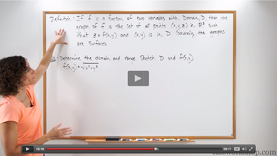
If $f$ is a function of two variables with domain $D$ , then the graph of $f$ is the set of all points $(x, y, z)$ in $R^{3}$ such that $z = f (x, y)$ and $(x, y)$ is in $D$ .

It may be helpful to think of it this way.

Imagine the graph of the surface, $S$ of $f$ , as lying directly above its domain $D$ in the xy-plane.

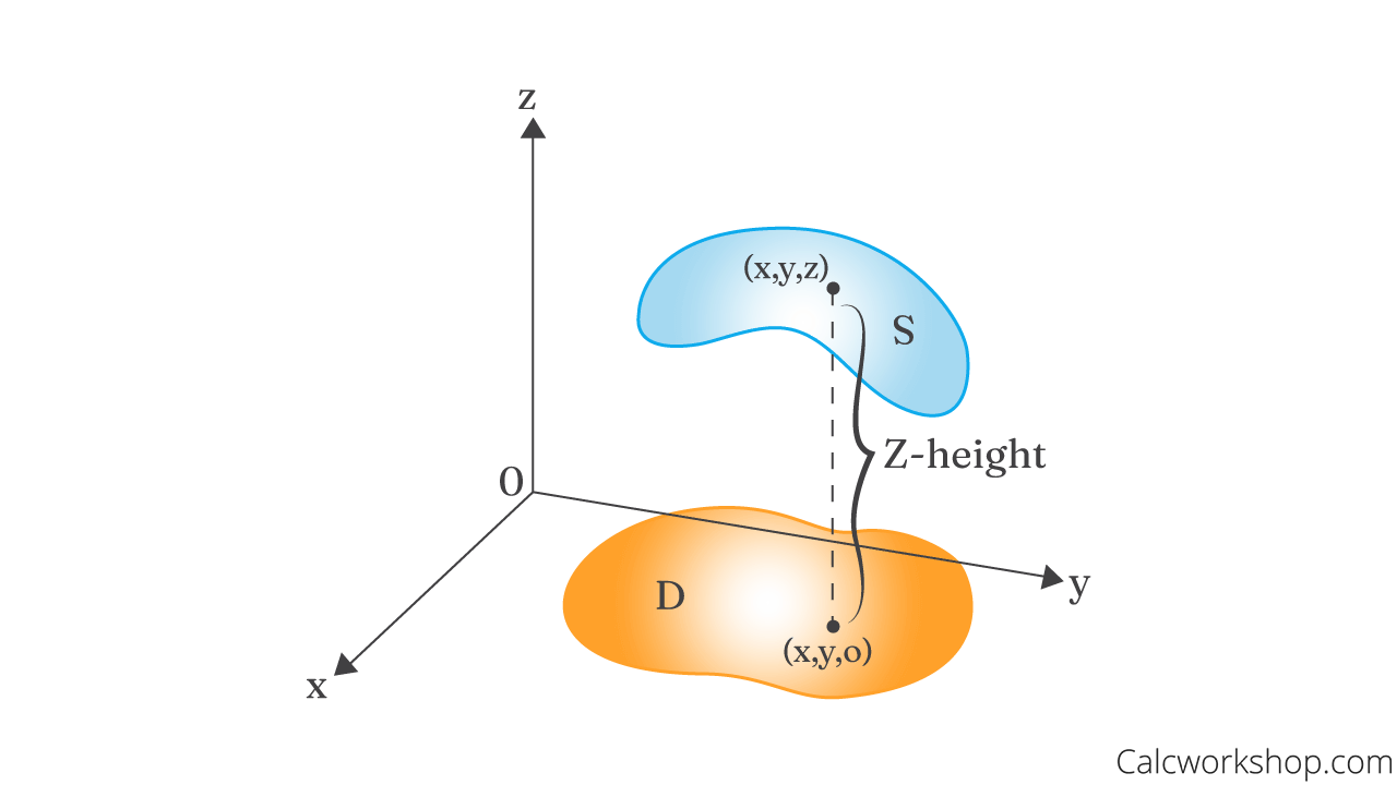
Surface Projected Domain

And the easiest way to create such a graph is by utilizing the method of level curves, sometimes called contour curves.

The level curves of a function $f$ of two variables are the curves with equations $f (x, y) = k$ , where $k$ is a constant and represents the set of all points in the domain of $f$ at which $f$ takes on a given value of $k$ .

But here’s what is important to note!

The level curves $f (x, y) = k$ are nothing more than the traces of the graph of $f$ in the horizontal plane $z = k$ projected down onto the xy-plane.

Example #1 – Sketch The Graph

For instance, suppose we are asked to sketch the graph $f (x, y) = \sqrt{25 - x^{2} - y^{2}}$ .

First, we let $z = f (x, y)$ such that $z = \sqrt{25 - x^{2} - y^{2}}$ .

Next, we will simplify our equation by squaring both sides to obtain a more recognizable function.

$\begin{aligned} z^{2} = 25 - x^{2} - y^{2} \\ x^{2} + y^{2} + z^{2} = 25 \end{aligned}$

Now, some of you may instantly recognize the function is the top half of a sphere (i.e., hemisphere) where $z \geq 0$ due to the square root, and with radius 5.

But for the rest of us, we still might need a bit more help.

Example #2 – Project Our Surface Onto The XY-Plane

Not to fear!

We simply create level curves to help us make sense of our surface.

Let $z = k$ , where $k$ is a constant, so we can project our surface onto the xy-plane.

$\begin{aligned} x^{2} + y^{2} + k^{2} = 25 \\ x^{2} + y^{2} = (25 - k^{2}) \end{aligned}$

Now, we have a circle, and if we plug in values for $k$ , such as $k = 0, 1, 2, 3, 4, 5$ and graph becomes:

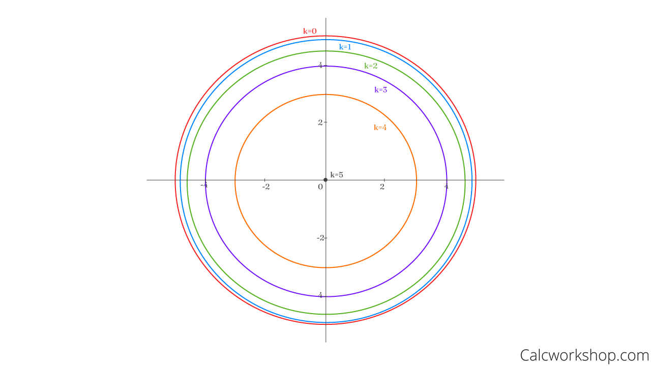
Sketching Level Curves

See, all we have to do is create a discrete set of height values by letting $z = k$ and then sketching the resulting curve in the xy-plane, and the shape is instantly more easily identifiable.

And lastly, we simply must visualize these level curves “lifted up” to form the surface in three-dimensional space.

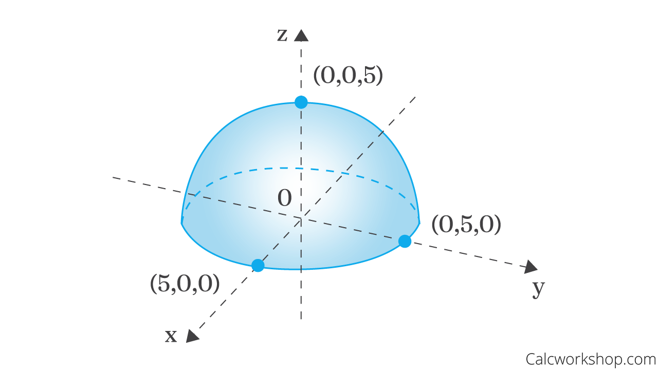
Level Curves 3D Surface

Together we will study the functions of several variables and explore how independent and dependent variables impact a function’s domain and range. And we will learn how graph level curves and surfaces for functions of two variables or more.

Let’s jump right in.

Video Tutorial w/ Full Lesson & Detailed Examples (Video)

functions-several-variables-example

Get access to all the courses and over 450 HD videos with your subscription

Monthly and Yearly Plans Available

Get My Subscription Now

Still wondering if CalcWorkshop is right for you?
Take a Tour and find out how a membership can take the struggle out of learning math.

4.9 / 5

1,143 Reviews

Shelby12-10-24 - OH, United States

CalcWorkshop was a wonderful resource as someone going onto a college calculus 1 class after not having taken a math course in a year! Jenn always explained things in a logical order that built upon previous lessons, and the way she explained topics was always easy to understand. Calcworkshop saved this semester for me, and I couldn't be more grateful to have found this site. :)

Jordan Q.12-09-24 - AR, United States

Anyone struggling with math at any level would greatly benefit from this product. I signed up for it immediately after getting a D on my first exam in calculus 2 and ended up getting A's and B's on the remaining exams, getting a B overall in the class. Jenn breaks down the topics, without skipping any steps, in a way that makes them very easy to understand. I highly recommend this product!

Dillon04-16-25 - SC, United States

I have been taking my college math courses online because I work full time. It was extremely hard for me to teach myself the material from the textbook without anyone explaining what needed to be done and it was trial, and error and I quickly fell behind in Calculus and Calculus 2. I discovered Calc Workshop a few weeks ago and gave it a try. I went back several courses to refresh what I've learned in the past and I already know more now than I ever did taking the course online. Jen does an amazing job of explaining the material, giving the formulas, and showing where the formulas come from so that you don't HAVE to memorize as much. She also gives helpful tips on how to memorize the rest. I have messaged to ask her several questions and she has responded before the end of the next day every time with exactly the answer I needed. I intend to use Calc Workshop throughout the rest of my college math.

Perry R.04-15-25 - GA, United States

Jenn thoroughly explains every move that she makes! She' s easy to understand and responds when emailed with questions! Jenn is saving my Differential Equations grade!

William M.04-15-25 - GA, United States

Calcworkshop was/is an excellent resource for anyone interested in or currently learning math. I started my Math degree at 26, spending absolutely 0 time doing math between 18 and then. I did not even know how to FOIL. The subscription got me up to speed pretty quick and then I used it for a few other courses. Couldn't recommend it enough

Joey M.04-14-25 - AZ, United States

They make the complex simple. They provide a systematic approach to ensure your success.

Patrick04-09-25 - NJ, United States

I went through the discrete math course prior to taking it at a university. Jen made difficult concepts easy to understand, leaving me well prepared for my Discrete college course.

Jon, C.04-06-25 - MD, United States

CalcWorkshop is a premier resource for any student seeking to understand, practice, and succeed within the vast areas of mathematics. I am impressed with the quality of instruction and practice problems offered by Jenn. As a engineering student, I always utilize Calcworkshop as a the "first stop" to really understand and gain confidence in the subject. I credit my success in Calculus to Jenn and CalcWorkshop and making me "smarter than the average bear."

Sayida S.04-03-25 - PA, United States

I absolutely love this subscription. At first I was iffy about spending the money, but in the long term it is so worth it. I started watching Jenn almost 3/4ths into my calc 2 class, and I a confidently say I understand the depths to each topic. Before, with my professor I felt that I only understood surface level of each topic. But after the CalcWorkshop videos, I have acronyms, tips, and knowledge I walk away with, that I didn't have before. Genuinely cannot wait to keep using this website for my future endeavors, minoring in Mathematics!

Gina K.03-30-25 - WA, United States

My experience was great! I needed help studying for my math class, but I wasn't sure how-until an ad for this popped up on my YouTube. After watching the ad, I was convinced, so I subscribed to CalcWoskop. I'm so happy I did because it helped me so much with my class! I learned a lot that I couldn't grasp from my college lectures, and this was the perfect solution.

Maria03-26-25 - AB, Canada

I found Jenn's videos near the end of my discrete math class, so I only had a month to go through all of her discrete math lessons to study for my exam. I'm sure I would have aced it if I had more time but I got a pretty good grade considering I thought I would fail.So happy to be done that class!As advertised, Jenn is very thorough and doesn't skip steps, she lets you know exactly how she gets from a to b or she will refer you to other videos where she teaches the techniques she's using more in depth. This was extremely valuable to me, being a mature student taking advanced math while not remembering basic algebra.And it was fun to understand and solve complex problems vs memorize proof structures.

RCJK03-07-25 - ID, United States

I had to take Calculus I and II as accelerated classes while working full time. It was my first time taking this courses and was very overwhelming. Calcworkshop really made learning the subjects easier for me by having all the subjects easy to find and easy to understand explanations. I received a B in both classes which I am extremely happy with doing the classes in double time.

Jacqueline S.03-07-25 - SC, United States

Jenn is awesome!Her breakdown of the topic is beyond what you would expect. She is showing you how to arrive at the answer instead of doing a simple equation. Most people need to know the why it give confidence and structure to the learning process. This is what Jenn is great at, she knows how to deliver the information to a non math mind in a way that instills knowledge that you can forever draw from as you move forward. It's really well thought out. She is a true master teacher. Thanks for all that you do for us! Hugs n Blessings... JS

Jujuana03-05-25 - MO, United States

I love the videos the way each lesson is explained step by step. I love that she has examples that you can go over again and again in order to understand the way algebra works. I was lost because my instructor was flying through each lesson and I was totally lost. I attached my syllabus and they helped me stay focus on what I was working and give me a guide to go back and refresh what I went over in class.

Stacey01-31-25 - AZ, United States

Hello, I highly recommend getting a subscription to Jenn and her Calcworkshop teaching math service. I did a general, "go from bad to good at math", Google search and found out about Calcworkshop through responses to the topic on reddit. I've just started watching her videos and found them to be extremely helpful. I'm going back to college after a long absence and math was never my strong suit. So I'm starting at the very bottom of her available subjects and going from there. Just watching a couple of the videos has taken me from being dragged along not understanding to following along just fine in my math class. I'm moving from the "I'll never get this", to the "I look forward to understanding this", mindset in approaching math. This for me is huge, and even though I have a long way to go, I'm confident I will get there thanks to Jenn. Totally worth it!

Kathy W.01-14-25 - WA, United States

Calcworkshop is an outstanding source to learn math and understanding math concepts. Jenn is an outstanding master teacher. Every lesson is clearly presented making understanding easy to grasp. Practice lessons with accompanying answers are given for each section. I am 82, a retired teacher and lifelong learner. Learning calculus has always been on my bucket list. Calcworkshop is helping me reach my goal.

Cheryl01-14-25 - NY, United States

Calc workshop is the absolutely best resource for math and I have seen almost everything that exists out there. I have even recommended it to my daughter's school so that all the kids could use the videos during the summer months for the subject they plan to study in the fall. They are guaranteed to get a A if they have watched the videos and completed the problems before taking the class. Students who are weak in areas can access lower level classes and those who seek to advance above grade level can do so. The videos and exercises are crystal clear and the excellent presentations raise the bar for teachers everywhere. I have always believed that one great math teacher is important in the education process. The videos, exercises and problems are excellent. It is not possible to have ANY knowledge gaps. I have never seen anything on the market that even begins to compete with it!

Justin N.12-22-24 - OK, United States

Calculus can be a scary subject. I know I was scared. I had been out of any math class for over 23 years. I had taken an 8 week Calculus 1 class and felt like I was overloaded. Going into Calculus 2 I found CALCWORKSHOP.com. I used the training videos and material to really dive back into Calc 1 and prepare for Calc 2. Long story short with the material provided and ample study time, I finished Calc 2 with a 95%. Thanks Jenn!