What if I told you that a matrix inherently produces two fundamental subspaces- Column and Null Space?
It’s true!
Understanding Subspaces and Spans
But first, let’s remember that a subspace of \(\mathbb{R}^{n}\) is a subset of vector space V satisfying the conditions that it contains the zero vector and is closed under addition and scalar multiplication.
And subspaces are spans, and spans are subspaces.
Meaning, if \(\overrightarrow{v_{1}}, \overrightarrow{v_{2}}, \ldots, \overrightarrow{v_{p}}\) are vectors in \(\mathbb{R}^{n}\).
Then \(\operatorname{Span}\left\{\overrightarrow{v_{1}}, \overrightarrow{v_{2}}, \ldots, \overrightarrow{v_{p}}\right\}\) is a subspace of \(\mathbb{R}^{n}\) and can be written as a span of a set of \(\mathrm{p}\) linearly independent vectors such that \(n \geq p\).
Column and Null Spaces in a Matrix
So, if \(\mathrm{A}\) is an \(m \times n\) matrix then the column space of \(\mathrm{A}\) is the subspace of \(\mathbb{R}^{m}\) spanned by the columns of \(\mathrm{A}\), denoted \(\operatorname{Col}(A)\).
Whereas the null space of an \(m \times n\) matrix \(\mathrm{A}\), denoted \(\operatorname{Nul}(A)\), is the subspace of \(\mathbb{R}^{n}\) consisting of all solutions of the homogeneous equation \(\overrightarrow{A x}=\overrightarrow{0}\).
Alright, so what does this really mean?
The column space and the null space of matrix A are both subspaces, so they are both spans.
The column space spans the columns of A and represents the “pivots columns.” The null space is the solution set of a homogeneous system of equations in parametric vector form, and represent the “free variables.”
Practical Example: Finding Column and Null Spaces
For example, let’s find a spanning set for the columns space and the null space for the matrix below.
\begin{align*}
A=\left[\begin{array}{ccccc}
-3 & 6 & -1 & 1 & -7 \\
1 & -2 & 2 & 3 & -1 \\
2 & -4 & 5 & 8 & -4
\end{array}\right]
\end{align*}
Our first step is to augment the matrix with the zero vector and calculate the reduced row echelon form (RREF).
\begin{equation}
\left[\begin{array}{cccccc}
-3 & 6 & -1 & 1 & -7 & 0 \\
1 & -2 & 2 & 3 & -1 & 0 \\
2 & -4 & 5 & 8 & -4 & 0
\end{array}\right] \sim\left[\begin{array}{cccccc}
1 & -2 & 0 & -1 & 3 & 0 \\
0 & 0 & 1 & 2 & -2 & 0 \\
0 & 0 & 0 & 0 & 0 & 0
\end{array}\right]
\end{equation}
Understanding Column Space
Notice that the first and third columns contain our pivots. Therefore we have found our column space, which is the span of these two columns from matrix A.
\begin{align*}
\operatorname{Col}(A)=\left\{\left[\begin{array}{c}
-3 \\
1 \\
2
\end{array}\right],\left[\begin{array}{c}
-1 \\
2 \\
5
\end{array}\right]\right\}
\end{align*}
Finding the Null Space
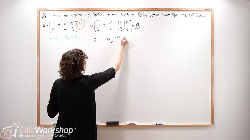
Now let’s write the general solution and notice that we have three free variables, namely \(x_{2}, x_{4}\), and \(x_{5}\).
\begin{equation}
\left[\begin{array}{cccccc}
1 & -2 & 0 & -1 & 3 & 0 \\
0 & 0 & 1 & 2 & -2 & 0 \\
0 & 0 & 0 & 0 & 0 & 0
\end{array}\right]
\end{equation}
\begin{aligned}
x_1-2 x_2-x_4+3 x_5 & = 0 \\
x_3+2 x_4-2 x_5 & = 0 \\
0 & = 0
\end{aligned}
\begin{aligned}
x_1 & = 2 x_2 + x_4 – 3 x_5 \\
x_2 & = x_2 \\
x_3 & = -2 x_4 + 2 x_5 \\
x_4 & = x_4 \\
x_5 & = x_5
\end{aligned}
Next, we write our solution in parametric vector form.
\begin{align*}
\left\{\begin{array}{c}
x_{1}=2 x_{2}+x_{4}-3 x_{5} \\
x_{2}=x_{2} \\
x_{3}=-2 x_{4}+2 x_{5} \\
x_{4}=x_{4} \\
x_{5}=x_{5}
\end{array} \rightarrow\left[\begin{array}{c}
x_{1} \\
x_{2} \\
x_{3} \\
x_{4} \\
x_{5}
\end{array}\right]=x_{2}\left[\begin{array}{l}
2 \\
1 \\
0 \\
0 \\
0
\end{array}\right]+x_{4}\left[\begin{array}{c}
1 \\
0 \\
-2 \\
1 \\
0
\end{array}\right]+x_{5}\left[\begin{array}{c}
-3 \\
0 \\
2 \\
0 \\
1
\end{array}\right]\right.
\end{align*}
So, the spanning set for the null space of matrix A is every linear combination of the vectors from our parametric form above.
\begin{align*}
\operatorname{Nul}(A)=\left\{\left[\begin{array}{l}
2 \\
1 \\
0 \\
0 \\
0
\end{array}\right],\left[\begin{array}{c}
1 \\
0 \\
-2 \\
1 \\
0
\end{array}\right],\left[\begin{array}{c}
-3 \\
0 \\
2 \\
0 \\
1
\end{array}\right]\right\}
\end{align*}
See, writing the column space and null space couldn’t be easier!
Remember, the spanning set for the null space is found by calculating the parametric vector form of the solutions to the homogeneous linear equations \(\mathrm{Ax}=0\), where the free variables form the spanning set for \(\operatorname{Nul}(\mathrm{A})\).
But there’s more.
Row Space of a Matrix
If \(\mathrm{A}\) is an \(m \times n\) matrix, each row of \(\mathrm{A}\) has \(\mathrm{n}\) entries and therefore can be identified with as a vector in \(\mathbb{R}^{n}\).
Moreover, the set of all linear combinations of the row vectors is called the row space of \(\mathrm{A}\), denoted \(\operatorname{Row}(A)\). And since each row has \(\mathrm{n}\) entries, \(\operatorname{Row}(A)\) is a subspace of \(\mathbb{R}^{n}\).
So, using our example the row space of matrix \(A\) is the subspace \(\mathbb{R}^{5}\) of spanned by \(\left\{\overrightarrow{r_{1}}, \overrightarrow{r_{2}}, \overrightarrow{r_{3}}\right\}\), such that \(\operatorname{Row} A=\operatorname{Span}\left\{\vec{r}_{1}, \overrightarrow{r_{2}}, \overrightarrow{r_{3}}\right\}\)
\begin{equation}
A=\left[\begin{array}{ccccc}
-3 & 6 & -1 & 1 & -7 \\
1 & -2 & 2 & 3 & -1 \\
2 & -4 & 5 & 8 & -4
\end{array}\right]
\end{equation}
\begin{equation}
\begin{array}{ll}
& \vec{r}_1=\left[\begin{array}{lllll}
-3 & 6 & -1 & 1 & -7
\end{array}\right] \\
\Leftrightarrow & \vec{r}_2=\left[\begin{array}{lllll}
1 & -2 & 2 & 3 & -1
\end{array}\right] \\
& \vec{r}_3=\left[\begin{array}{lllll}
2 & -4 & 5 & 8 & -4
\end{array}\right]
\end{array}
\end{equation}
Determining the Row Space of a Matrix
But how do we determine the row space of a matrix?
Well, all we have to do is reduce A to echelon form (REF) and identify our pivot rows.
Practical Example: Finding Column, Null, and Row Spaces
Alright, so let’s find the spanning set for the column space, null space, and row space for the matrix below.
\begin{align*}
A=\left[\begin{array}{ccccc}
-2 & -5 & 8 & 0 & -17 \\
1 & 3 & -5 & 1 & 5 \\
3 & 11 & -19 & 7 & 1 \\
1 & 7 & -13 & 5 & -3
\end{array}\right]
\end{align*}
First, we augment and reduce our matrix to echelon form (REF).
\begin{align*}
A \sim B:\left[\begin{array}{cccccc}
-2 & -5 & 8 & 0 & -17 & 0 \\
1 & 3 & -5 & 1 & 5 & 0 \\
3 & 11 & -19 & 7 & 1 & 0 \\
1 & 7 & -13 & 5 & -3 & 0
\end{array}\right] \sim\left[\begin{array}{cccccc}
1 & 3 & -5 & 1 & 5 & 0 \\
0 & 1 & -2 & 2 & -7 & 0 \\
0 & 0 & 0 & -4 & 20 & 0 \\
0 & 0 & 0 & 0 & 0 & 0
\end{array}\right]
\end{align*}
Identifying Column and Row Spaces
Now we identify our column space, the pivot columns from the original matrix A.
\begin{align*}
\text { ColA }=\left\{\left[\begin{array}{c}
-2 \\
1 \\
3 \\
1
\end{array}\right],\left[\begin{array}{c}
-5 \\
3 \\
11 \\
7
\end{array}\right],\left[\begin{array}{l}
0 \\
1 \\
7 \\
5
\end{array}\right]\right\}
\end{align*}
And our row space which are the rows that contain our pivots of our transformed matrix B.
\begin{align*}
\text { RowA }=\left\{\left[\begin{array}{lllll}
1 & 3 & -5 & 1 & 5
\end{array}\right],\left[\begin{array}{lllll}
0 & 1 & -2 & 2 & -7
\end{array}\right],\left[\begin{array}{lllll}
0 & 0 & 0 & -4 & 20
\end{array}\right]\right\}
\end{align*}
Next, we continue our elementary row operations to reduced row echelon form (RREF).
\begin{equation}
A \sim B \sim C:\left[\begin{array}{cccccc}
-2 & -5 & 8 & 0 & -17 & 0 \\
1 & 3 & -5 & 1 & 5 & 0 \\
3 & 11 & -19 & 7 & 1 & 0 \\
1 & 7 & -13 & 5 & -3 & 0
\end{array}\right]
\end{equation}
\begin{equation}
\underset{R E F}{\sim}\left[\begin{array}{cccccc}
1 & 3 & -5 & 1 & 5 & 0 \\
0 & 1 & -2 & 2 & -7 & 0 \\
0 & 0 & 0 & -4 & 20 & 0 \\
0 & 0 & 0 & 0 & 0 & 0
\end{array}\right]
\end{equation}
\begin{equation}
\underset{R R E F}{\sim}\left[\begin{array}{cccccc}
1 & 0 & 1 & 0 & 1 & 0 \\
0 & 1 & -2 & 0 & 3 & 0 \\
0 & 0 & 0 & 1 & -5 & 0 \\
0 & 0 & 0 & 0 & 0 & 0
\end{array}\right]
\end{equation}
Finding the General and Parametric Forms
Now we find our general form and parametric form.
\begin{align*}
\left\{\begin{array}{c}
x_{1}=-x_{3}-x_{5} \\
x_{2}=2 x_{3}-3 x_{5} \\
x_{3}=x_{3} \\
x_{4}=5 x_{5} \\
x_{5}=x_{5}
\end{array} \rightarrow\left[\begin{array}{l}
x_{1} \\
x_{2} \\
x_{3} \\
x_{4} \\
x_{5}
\end{array}\right]=x_{3}\left[\begin{array}{c}
-1 \\
2 \\
1 \\
0 \\
0
\end{array}\right]+x_{5}\left[\begin{array}{c}
-1 \\
-3 \\
0 \\
5 \\
1
\end{array}\right]\right.
\end{align*}
Concluding the Null Space
Thus, the null space for matrix \(A\) is as follows
\begin{align*}
N u l A=\left\{\left[\begin{array}{c}
-1 \\
2 \\
1 \\
0 \\
0
\end{array}\right],\left[\begin{array}{c}
-1 \\
-3 \\
0 \\
5 \\
1
\end{array}\right]\right\}
\end{align*}
Awesome!
And subspace of vectors can be described in terms of a linear transformation instead of matrices.
A linear transformation \(\mathrm{T}\) from a vector space \(\mathrm{V}\) into a vector space \(\mathrm{W}\) is a rule that assigns to each vector \(\mathrm{x}\) in \(\mathrm{V}\) a unique vector \(T(\vec{x})\) in \(\mathrm{W}\) such that:
- T(u+v) = T(u) + T(v) for all u and v in V.
- T(cu) = cT(u) for all u in V and all scalars c.
And the kernel (null space) of \(\mathrm{T}\) is the set of all \(\mathrm{u}\) in \(\mathrm{V}\) such that:
\begin{equation}
T(\vec{u})=\overrightarrow{0}
\end{equation}
The process and steps are the same. Only we need to create our matrix by constructing a set of linear combinations of the vectors given.
In this video, you will:
- See various concepts in action, making them easier to understand
- Determine if a vector is in the null space
- Find matrix A given the column space
- Define linear transformations for polynomials
- Describe the kernel and range of T
- Determine whether a vector is in the ColA, NulA, or both
Get ready to explore these concepts, and let’s dive in!
Video Tutorial w/ Full Lesson & Detailed Examples
Get access to all the courses and over 450 HD videos with your subscription
Monthly and Yearly Plans Available
Still wondering if CalcWorkshop is right for you?
Take a Tour and find out how a membership can take the struggle out of learning math.