Now that we know how to represent vector spaces and subspaces, it is time to find a basis of a subspace as a coordinate system.
The Concept of a Coordinate System
What’s a coordinate system, you may ask?
A coordinate system is a one-to-one mapping of the points in a set into \(\mathbb{R}^{n}\).
All this means is that we are giving directions to our points.
Suppose we are working in the \(2 \mathrm{D}\) coordinate plane with ordered pairs \((\mathrm{x}, \mathrm{y})\).
The \(\mathrm{x}\) coordinate tells us to move left or right (east or west), and the y-coordinate tells us how much to move up or down (north or south).
Vector Coordinate System
The same thing happens with the vector coordinate system but with a twist.
Working with Basis and B-Coordinates
Assume \(\beta=\left\{\vec{b}_{1}, \ldots, \vec{b}_{n}\right\}\) is a basis for vector space \(\mathrm{V}\) and \(\vec{x}\) is in \(\mathrm{V}\).
The coordinates of \(\vec{x}\) relative to the basis \(\beta\), sometimes called the B-Coordinates of \(\mathrm{x}\), are the unique weights (scalars) such that \(\vec{x}=c_{1} \overrightarrow{b_{1}}+\ldots+c_{n} \overrightarrow{b_{n}}\) and the \(\mathrm{B}\)-coordinate vector of \(\mathrm{x}\) is the vector.
\begin{align*}
[\vec{x}]_{\beta}=\left[\begin{array}{c}
c_{1} \\
\vdots \\
c_{n}
\end{array}\right] \text { in } \mathbb{R}^{n}
\end{align*}
Therefore, the coordinates of \(\mathrm{V}\) are the coefficients!
Let’s see this in action.
Practical Example: Calculating Vector Coordinates
Consider a basis \(\beta=\left\{\overrightarrow{b_{1}}, \overrightarrow{b_{2}}\right\}\) for \(\mathbb{R}^{2}\).
Where \(\overrightarrow{b_{1}}=\left[\begin{array}{l}1 \\ 0\end{array}\right]\) and \(\overrightarrow{b_{2}}=\left[\begin{array}{l}2 \\ 1\end{array}\right]\).
Suppose an \(\vec{x}\) in \(\mathbb{R}^{2}\) has the coordinate vector \([\vec{x}]_{\beta}=\left[\begin{array}{l}3 \\ 5\end{array}\right]\). Find \(\vec{x}\).
First, we will note that the B-coordinate vector is simply our coefficients.
\begin{aligned}
\left[\begin{array}{c}
x
\end{array}\right]_{\beta} & =\left[\begin{array}{l}
c_{1} \\
c_{2}
\end{array}\right]=\left[\begin{array}{l}
3 \\
5
\end{array}\right]
\end{aligned}
Therefore, we can write our linear combination as seen below and calculate our vector:
\begin{aligned}
\vec{x} & =c_{1} \vec{b}_{1}+\ldots+c_{n} \vec{b}_{n} \\
& =3\left[\begin{array}{l}
1 \\
0
\end{array}\right]+5\left[\begin{array}{l}
2 \\
1
\end{array}\right] \\
& =\left[\begin{array}{l}
3 \\
0
\end{array}\right]+\left[\begin{array}{c}
10 \\
5
\end{array}\right] \\
& =\left[\begin{array}{c}
13 \\
5
\end{array}\right]
\end{aligned}
Easy!
Notice that the entries in the vector \(\vec{x}=\left[\begin{array}{c}13 \\ 5\end{array}\right]\) are the coordinates of \(\vec{x}\) relative to the “standard basis” \(E=\left\{\overrightarrow{e_{1}}, \overrightarrow{e_{2}}\right\}\).
Since \(\left[\begin{array}{c}13 \\ 5\end{array}\right]=13\left[\begin{array}{l}1 \\ 0\end{array}\right]+5\left[\begin{array}{l}0 \\ 1\end{array}\right]=13 e_{1}+5 e_{2}\)
In other words, if we start at the origin, we will travel 13 units to the right (east) and 5 units up (north).
But what if you want to find the B-coordinate vector?
Thankfully this can be easily found using the change of coordinate matrix \(P_{\beta}\).
If \(P_{\beta}=\left[\begin{array}{llll}\overrightarrow{b_{1}} & \vec{b}_{2} & \cdots & \overrightarrow{b_{n}}\end{array}\right]\) and \(\vec{x}=c_{1} \vec{b}_{1}+\ldots+c_{n} \vec{b}_{n}\).
Then \(\vec{x}=P_{\beta}[\vec{x}]_{\beta}\)
Thus, if we want to find \(\vec{x}\) we multiply and if we want to find \([\vec{x}]_{\beta}\) we augment our matrix \(P_{\beta}\) with \(\vec{x}\) and row reduce, \(\left[P_{\beta} \quad \vec{x}\right]\).
For example, let’s find the coordinate vector \([\vec{x}]_{\beta}\) of \(\vec{x}=\left[\begin{array}{c}-2 \\ 1\end{array}\right]\) relative to the basis \(\beta=\left\{\vec{b}_{1}, \overrightarrow{b_{2}}\right\}\).
Where \(\overrightarrow{b_{1}}=\left[\begin{array}{c}1 \\ -3\end{array}\right]\) and \(\overrightarrow{b_{2}}=\left[\begin{array}{c}2 \\ -5\end{array}\right]\).
First, we will write our given basis in coordinate matrix form.
\begin{aligned}
P_{\beta} & =\left[\begin{array}{ll}
\overrightarrow{b_{1}} & \overrightarrow{b_{2}}
\end{array}\right] \\
& =\left[\begin{array}{cc}
1 & 2 \\
-3 & -5
\end{array}\right]
\end{aligned}
Next, we are looking for the B-coordinate matrix. We will first augment and row reduce.
\begin{aligned}
[\vec{x}]_{\beta} & =\left[\begin{array}{ll}
P_{\beta} & \vec{x}
\end{array}\right] \\
& =\left[\begin{array}{ccc}
1 & 2 & -2 \\
-3 & -5 & 1
\end{array}\right] \\
& \sim\left[\begin{array}{ccc}
1 & 0 & 8 \\
0 & 1 & -5
\end{array}\right]
\end{aligned}
So, \([\vec{x}]_{\beta}=\left[\begin{array}{c}8 \\ -5\end{array}\right]\)
Not too bad, right?
Alright, so to quickly recap.
What we’ve seen if \(\beta=\left\{\vec{b}_{1}, \ldots, \overrightarrow{b_{n}}\right\}\) is a basis for a subspace \(\mathrm{V}\), then all we have to do to find the B-coordinate vector is to solve the vector equation \(\vec{x}=c_{1} \vec{b}_{1}+\ldots+c_{n} \vec{b}_{n}\) by augmenting and row reducing.
Therefore, if \(\mathrm{x}\) is not in \(\mathrm{V}\), then the equation has no solution (i.e., the matrix is inconsistent).
Understanding Coordinate Mapping and Isomorphism
Now this leads us to the coordinate mapping of polynomials. But to do this, we must learn a new term: isomorphism.
A one-to-one linear transformation from a vector space \(\mathrm{V}\) onto a vector space \(\mathrm{W}\) is called an isomorphism from \(\mathrm{V}\) onto \(\mathrm{W}\).
Therefore, an isomorphism is a bijection, as it is both one-to-one (injective) and onto (surjective), as it preserves the basic properties of a subspace.
Huh?
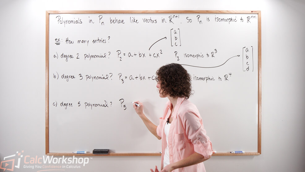
Isomorphism in Degree 2 Polynomials
Isomorphism means “the same.” Consequently, if we are talking about a polynomial of degree 2, then this is isomorphic, the same as dealing with \(\mathbb{R}^{3}\), as a degree two polynomial has up to three terms.
\begin{align*}
P_{2} \rightarrow \mathbb{R}^{3}: c+b x+a x^{2} \mapsto\left[\begin{array}{l}
c \\
b \\
a
\end{array}\right]
\end{align*}
Practical Example: Spanning Set of Polynomials
For example, suppose we want to determine if a set of polynomials, such as \(\left\{5 t+t^{2}, 1-8 t-2 t^{2},-3+4 t+2 t^{2}, 2-3 t\right\}\) spans \(P_{2}\).
First, we recognize that \(P_{2}\) means “degree 2 polynomial.” Thus, \(P_{2}\) is isomorphic to \(R^{3}\).
\begin{aligned}
\left\{0+5 t+t^{2},\right. & \\
\left. 1-8 t-2 t^{2},\right. & \\
\left. -3+4 t+2 t^{2},\right. & \\
\left. 2-3 t+0 t^{2}\right\} & \\
& \Rightarrow \left[\begin{array}{cccc}
0 & 1 & -3 & 2 \\
5 & -8 & 4 & -3 \\
1 & -2 & 2 & 0
\end{array}\right]
\end{aligned}
Now we create a matrix and row reduce. If the set spans \(P_{2}\), then it will contain 3 pivots. If the matrix doesn’t include the necessary number of pivots, then it does not span.
\begin{align*}
\left[\begin{array}{cccc}
0 & 1 & -3 & 2 \\
5 & -8 & 4 & -3 \\
1 & -2 & 2 & 0
\end{array}\right] \sim\left[\begin{array}{cccc}
1 & 0 & -4 & 0 \\
0 & 1 & -3 & 0 \\
0 & 0 & 0 & 1
\end{array}\right]
\end{align*}
Therefore, because we have 3 pivots, we know that the set of polynomials does indeed span \(P_{2}\).
See, not hard at all.
Introduction to Vector Space Dimensions and the Basis Theorem
Okay, now it’s time to talk about the dimensions of vector spaces and the Basis Theorem.
If a vector space \(\mathrm{V}\) has a basis \(\beta=\left\{\vec{b}_{1}, \ldots, \vec{b}_{n}\right\}\) then any set in \(\mathrm{V}\) containing more than n vectors must be linearly dependent.
Conversely, if a vector space \(\mathrm{V}\) has a basis of \(\mathrm{n}\) vectors, then every basis of \(\mathrm{V}\) must consist of exactly \(\mathrm{n}\) vectors.
Therefore, if we let \(\mathrm{H}\) be a subspace of a finite-dimensional vector space \(\mathrm{V}\). Any linearly independent set in \(\mathrm{H}\) can be expanded, if necessary, to a basis for \(\mathrm{H}\) as \(\operatorname{dim} H \leq \operatorname{dim} V\)
Practical Example: Subspaces of \(R^{3}\) and the Basis Theorem
For example, the subspaces of \(R^{3}\) can be any of the following dimensions:
- 0 -dimensional subspaces (only the zero subspace)
- 1-dimensional subspaces (any subspace spanned by a single nonzero vector, such as lines through the origin)
- 2-dimensional subspaces (any subspace spanned by two linearly independent vectors, such as planes through the origin)
- 3-dimensional subspaces (any three linearly independent vectors in \(R^{3}\) that span all of \(R^{3}\))
Hence, the Basis Theorem states that if we let \(\mathrm{V}\) be a \(\mathrm{p}\)-dimensional vector space where \(p \geq 1\). Any linearly independent set of exactly \(\mathrm{p}\) elements in \(\mathrm{V}\) is automatically a basis for \(\mathrm{V}\). And any set of exactly \(\mathrm{p}\) elements that spans \(\mathrm{V}\) is automatically a basis for \(\mathrm{V}\).
Importance of the Basis Theorem and Understanding the Dimensions
Why is this important?
Because the dimension of the null space, denoted \(\operatorname{dim} N u l A\), is the number of free variables in the equation \(\overrightarrow{A x}=\overrightarrow{0}\) and the dimensions of the columns space, denoted \(\operatorname{dim} \operatorname{Col} A\), is the number of pivot columns in \(\mathrm{A}\)
Cool!
Next Steps
In this lesson, you will:
- Dig deeper into the understanding of the dimensions of a vector space
- Make connections to the Invertible Matrix Theorem, Spanning Set Theorem, and Basis Theorem
- Revisit polynomials and transformations
- Grasp the idea behind isomorphisms
- Revisit the null space, column space, and row space
Get ready for a wild ride!
Video Tutorial w/ Full Lesson & Detailed Examples
Get access to all the courses and over 450 HD videos with your subscription
Monthly and Yearly Plans Available
Still wondering if CalcWorkshop is right for you?
Take a Tour and find out how a membership can take the struggle out of learning math.