Change of Basis
The Ultimate Vector Transformation

Have you ever wondered whether bases are helpful?

Understanding the Concept of a Change of Basis

Well, the change of basis, also referred to as the change of coordinate matrix from \(\mathrm{B}\) to \(\mathrm{C}\), will convince you of its usefulness.

As we have discovered, if \(\mathrm{V}\) is a vector space with basis \(B=\left\{\vec{b}_{1}, \ldots, \overrightarrow{b_{n}}\right\}\) then every element \(\vec{x}\) in \(\mathrm{V}\) can be written uniquely as a linear combination of the basis elements such that:

\begin{equation}
\vec{x}=c_1 \overrightarrow{b_1}+c_2 \overrightarrow{b_2}+\cdots+c_n \overrightarrow{b_n}
\end{equation}

Where the scalars \(c_{i}\) can be denoted as a column vector of \(\vec{x}\) with respect to the basis \(\mathrm{B}\) known as the \(\mathrm{B}\)-coordinate vector of \(\vec{x}\).

What’s important is that every vector \(\vec{x}\) corresponds to exactly one such column vector in \(\mathbb{R}^{n}\), as we learned from our lesson on Coordinate Systems.

In particular, our study of isomorphisms showed us how sets of polynomials can “match” elements of \(V\) and \(\mathbb{R}^{n}\).

Consequently, by choosing a basis, a vector space of dimension \(\mathrm{n}\) can be easily identified with \(\mathbb{R}^{n}\).

Why Choose a Different Basis?

I think we can all agree that this is very useful indeed. But what if we want to choose a different basis?

First, let’s talk about why we want to choose a different basis.

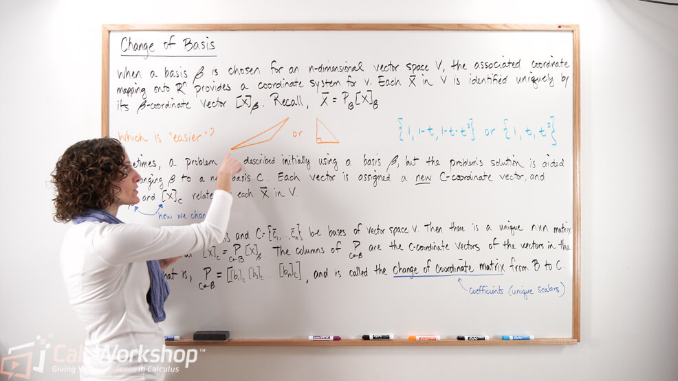
From the two images below, which one would be easier to calculate the perimeter and area?

Indeed, the square on the left is infinitely easier to analyze than the polygon on the right. Choosing the easier of the two shapes is always the most advisable.

Likewise, I think we’d all jump at the chance to work with an easier or more simplified vector space.

And that’s the idea of change of basis. We will change or transform a “hard” basis for one that is “easier.”

Because sometimes we aren’t given a nice “easy” square, but rather something a little unwieldy.

So, if we’re presented initially with a basis B, but the problem’s solution will be significantly aided by changing \(\mathrm{B}\) to a new basis \(\mathrm{C}\), then it’s advantageous for us to choose the bases that give the best matrix for our linear transformation.

And how is this accomplished?

The Mechanics of Change of Basis

If we let
\begin{aligned}
B & =\left\{\vec{b}_{1}, \ldots, \overrightarrow{b_{n}}\right\} \\
C & =\left\{\vec{c}_{1}, \ldots, \overrightarrow{c_{n}}\right\}
\end{aligned}
be bases of a vector space \(V\).

Then there is a unique \(n \times n\) matrix \(\underset{C \leftarrow B}{P}\) such that:

\begin{aligned}
[\vec{x}]_C & =\underset{C \leftarrow B}{P}[\vec{x}]_B
\end{aligned}

Where the columns of \(\underset{C \leftarrow B}{P}\) are the C-coordinate vectors of the vectors in the basis B.

Therefore,
\begin{aligned}
[\vec{x}]_B & =(\underset{C \leftarrow B}{P})^{-1}[\vec{x}]_{C}
\end{aligned}
by the invertible matrix theorem.

A Practical Example of Change of Basis

Consider two bases
\begin{aligned}
B & =\left\{\overrightarrow{b_{1}}, \overrightarrow{b_{2}}\right\} \\
C & =\left\{\overrightarrow{c_{1}}, \overrightarrow{c_{2}}\right\}
\end{aligned}
for a vector space \(\mathrm{V}\), such that:

\begin{aligned}
\overrightarrow{b_{1}} & =2 \overrightarrow{c_{1}}-3 \overrightarrow{c_{2}} \\
\overrightarrow{b_{2}} & =5 \overrightarrow{c_{1}}+4 \overrightarrow{c_{2}} \\
\vec{x} & =\overrightarrow{b_{1}}+3 \overrightarrow{b_{2}}
\end{aligned}

Let’s find \([\vec{x}]_{C}\).

First, we will write our change of basis matrix, \({ }_{C \leftarrow B}^{P}\), and our B-coordinate matrix from our given information.

\begin{aligned}
\left.\begin{array}{l}
\overrightarrow{b_1} &= 2 \overrightarrow{c_1} – 3 \overrightarrow{c_2} \\
\overrightarrow{b_2} &= 5 \overrightarrow{c_1} + 4 \overrightarrow{c_2}
\end{array}\right\}
\end{aligned}

\begin{aligned}
\underset{C \leftarrow B}{P} &= \left[\begin{array}{cc}
2 & 5 \\
-3 & 4
\end{array}\right]
\end{aligned}

\begin{aligned}
\vec{x} &= \vec{b}_1 + 3 \vec{b}_2 \\
\rightarrow[\vec{x}]_B &= \left[\begin{array}{l}
1 \\
3
\end{array}\right]
\end{aligned}

Next, we will multiply our matrices to find the C-coordinate matrix of \(\mathrm{x}\).

\begin{aligned}
[\vec{x}]_C &= \underset{C \leftarrow B}{P}[\vec{x}]_B \\
\Rightarrow [\vec{x}]_C &= \\
&= \left[\begin{array}{cc}
2 & 5 \\
-3 & 4
\end{array}\right] \left[\begin{array}{l}
1 \\
3
\end{array}\right] \\
&= \left[\begin{array}{c}
17 \\
9
\end{array}\right]
\end{aligned}

Easy, right?

Case Study: Finding C-Coordinate Matrix Without B-Coordinate

But what happens if we don’t have the B-coordinate matrix?

Well, we’ll use a similar strategy of the inverse algorithm given the theorem
\begin{aligned}
\left[\begin{array}{ll|ll}c_{1} & c_{2} & b_{1} & b_{2}\end{array}\right] & \sim\left[\begin{array}{l|l}I & \underset{C \leftarrow B}{P}\end{array}\right]
\end{aligned}
For example, suppose two bases
\begin{aligned}
B & =\left\{\vec{b}_{1}, \overrightarrow{b_{2}}\right\} \\
C & =\left\{\overrightarrow{\left.c_{1}, \overrightarrow{c_{2}}\right\}}\right.
\end{aligned}
for \(\mathbb{R}^{2}\) given by
\begin{aligned}
\overrightarrow{b_{1}} & =\left[\begin{array}{c}-3 \\ 1\end{array}\right] \\
\overrightarrow{b_{2}} & =\left[\begin{array}{c}4 \\ -2\end{array}\right] \\
\overrightarrow{c_{1}} & =\left[\begin{array}{c}9 \\ -7\end{array}\right] \\
\overrightarrow{c_{2}} & =\left[\begin{array}{c}7 \\ -5\end{array}\right]
\end{aligned}
and the change of coordinates matrix for \(\mathrm{B}\) to \(\mathrm{C}\) and the change of coordinates matrix from \(\mathrm{C}\) to \(\mathrm{B}\).

First, we create our augmented matrix and row reduce so that the Identity matrix is in front and our change of basis from \(\mathrm{B}\) to \(\mathrm{C}\) is in the back.

\begin{aligned}
\left[\begin{array}{llll}
c_{1} & c_{2} & b_{1} & b_{2}
\end{array}\right] &\sim\left[\begin{array}{cc}
I & P \\
C \leftarrow B
\end{array}\right] \\
&=\left[\begin{array}{cccc}
9 & 7 & -3 & 4 \\
-7 & -5 & 1 & -2
\end{array}\right] \\
&\sim\left[\begin{array}{cccc}
1 & 0 & 2 & -3 / 2 \\
0 & 1 & -3 & 5 / 2
\end{array}\right]
\end{aligned}

So, we just found the change of coordinate matrix from B to C, or the old basis relative to the new basis, by using Row Reduction as

\begin{aligned}
\underset{C \leftarrow B}{P} &= \left[\begin{array}{cc}
2 & -3 / 2 \\
-3 & 5 / 2
\end{array}\right]
\end{aligned}

Now, let’s find the change of the coordinates matrix from C to B. We have two choices… we can apply the algorithm as we did above, or we can use the Invertible Matrix Theorem to our advantage, knowing that \({ }_{B \leftarrow C}=(\underset{C \leftarrow B}{P})^{-1}\)

Let’s use inverses!

\begin{aligned}
\underset{B \leftarrow C}{P} &= (\underset{C \leftarrow B}{P})^{-1} \\
\Rightarrow \underset{B \leftarrow C}{P} &= \frac{1}{(1 / 2)}\left[\begin{array}{cc}
5 / 2 & 3 / 2 \\
3 & 2
\end{array}\right] \\
&= \left[\begin{array}{ll}
5 & 3 \\
6 & 4
\end{array}\right]
\end{aligned}

Sweet!

Next Steps

In this video, you will:

• Learn how to find a new basis C
• Find the Change-of-Coordinate Matrix from \(\mathrm{B}\) to \(\mathrm{C}\) and vice-versa
• Study the relationship between the B-Coordinate vector and the C-Coordinate vector
• Examine more examples dealing with the Change of Basis problem
• Revisit polynomials and find the Change-of-Coordinate Matrix for them

Get ready to change things up!

Video Tutorial w/ Full Lesson & Detailed Examples

Get access to all the courses and over 450 HD videos with your subscription

Monthly and Yearly Plans Available

Get My Subscription Now

Still wondering if CalcWorkshop is right for you?
Take a Tour and find out how a membership can take the struggle out of learning math.