What is a vector field?

Jenn, Founder Calcworkshop®, 15+ Years Experience (Licensed & Certified Teacher)
A vector field issues a vector to each point in space; thus, allowing us to represent physical occurrences we experience in our daily lives.
Vector fields, for instance, explain forces such as wind and water currents in the ocean, which are directly related to navigation. They also explain electric fields, force fields, and gravity on Earth.
The spinning effect of a merry-go-round or the sloshing of your morning cup of coffee illustrate the mechanics of vector fields.
They’re everywhere!
Vector Fields Defined
So, how do we define them?
In Two-Space
Let D be a set in \({\mathbb{R}^2}\) (plane region).
A vector field in \({\mathbb{R}^2}\) is a function \(\overrightarrow F \) that assigns to each point \(\left( {x,y} \right)\) in the domain \(D\) a two-dimensional vector:
\begin{equation}
\vec{F}(x, y)=\langle P(x, y), Q(x, y)\rangle
\end{equation}
where \(P\) and \(Q\) are functions of two variables.
In Three-Space
Let \(E\) be a set in \({\mathbb{R}^3}\).
A vector field in \({\mathbb{R}^3}\) is a function \(\overrightarrow F \) that assigns to each point \(\left( {x,y,z} \right)\) in the domain \(E\) a three-dimensional vector:
\begin{equation}
\vec{F}(x, y, z)=\langle P(x, y, z), Q(x, y, z), R(x, y, z)\rangle
\end{equation}
where \(P\), \(Q\), and \(R\) are functions of three variables.
All this means is that a vector field on a domain is a function that assigns a vector to each point in space, such that the input is a point and the output is a vector.
Graphing Vector Fields
So, how do we represent or graph these vector fields?
The graph of a vector field is created by plotting arrows one at a time by substituting points into the plane to determine what arrow to draw at that point.
Please note that graphing vector fields, especially 3D vector fields, are challenging and not easily sketched by hand. Therefore, we tend to rely on computers to generate graphs for us.
But that doesn’t mean that we can’t sketch some 2D vector fields to help us imagine the overall look of the vector field to determine some general characteristics. Such as,
- Do all the arrows point in the same direction?
- Do the vectors point directly towards or directly away from the origin?
- Do the lengths of the vectors remain constant, or do they increase or decrease as we move away from the origin?
Keep in mind that a vector field cannot be represented by one single curve or surface. Instead, we plot a sample of vectors to give us the general idea of the appearance of the vector field.
Please note that our focus will be on how to graph two-dimensional vector fields not three-dimensional vector fields, as 3D vector fields are best represented using computer software.
Example
Let’s look at a few examples of vector fields in \({\mathbb{R}^2}\).
Problem #1
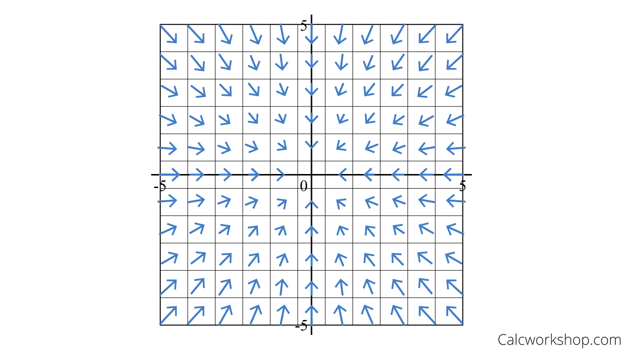
Graph \(\vec{F}(x, y)=\langle-x,-y\rangle\)
All we have to do is create a table and plug-in points by choosing a few points from each quadrant. Remember, we plug-in points (input), and it will spit out a vector (output).
\begin{equation}
\begin{array}{c|c}
\text { Points: }(x, y) & \text { Vectors: } \vec{F}(x, y)=\langle-x,-y\rangle \\
\hline(1,0) & \vec{F}(1,0)=\langle-1,0\rangle \\
\hline(0,1) & \vec{F}(0,1)=\langle 0,-1\rangle \\
\hline(1,1) & \vec{F}(1,1)=\langle-1,-1\rangle \\
\hline(3,2) & \vec{F}(3,2)=\langle-3,-2\rangle \\
\hline(-2,5) & \vec{F}(-2,5)=\langle-(-2),-5\rangle=\langle 2,-5\rangle \\
\hline \vdots & \vdots
\end{array}
\end{equation}Now, all that is left for us to do is to go to each input point and graph its associated vector. The graph of all of our outputs is our vector field.
Vector Field Pointing Toward Origin
Notice how all the arrows are pointing toward the origin and how the vectors increase in size the further we move away from the origin.
Problem #2
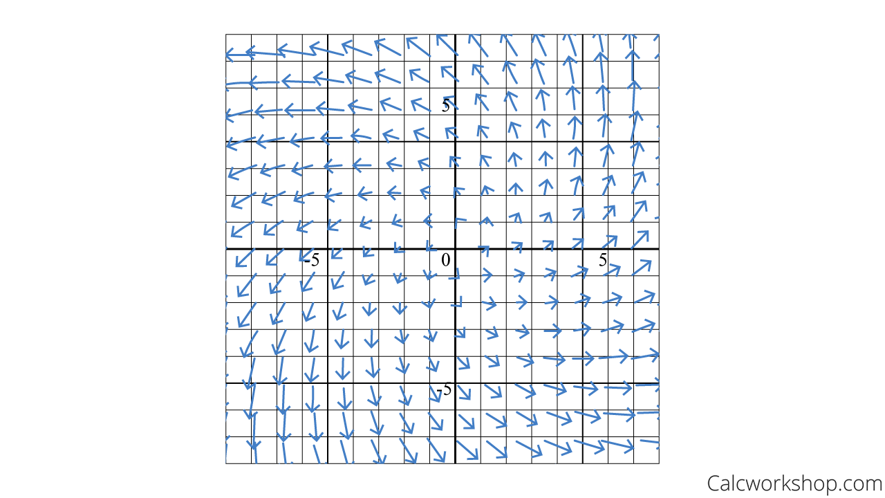
Graph \(\vec{F}(x, y)=\langle x-y, x+y\rangle\)
First, we create a table and plug-in points, ensuring we choose a few points from each quadrant. And note that the more points you plug in, the more accurate your sketch will be.
\begin{equation}
\begin{array}{c|c}
\text { Points: }(x, y) & \text { Vectors: } \vec{F}(x, y)=\langle x-y, x+y\rangle \\
\hline(1,0) & \vec{F}(1,0)=\langle 1-0,1+0\rangle=\langle 1,1\rangle \\
\hline(0,-1) & \vec{F}(0,-1)=\langle 0-(-1), 0+(-1)\rangle=\langle 1,-1\rangle \\
\hline(1,1) & \vec{F}(1,1)=\langle 1-1,1+1\rangle=\langle 0,2\rangle \\
\hline(-2,-3) & \vec{F}(-2,-3)=\langle-2-(-3),-2+(-3)\rangle=\langle 1,-5\rangle \\
\hline \vdots & \vdots
\end{array}
\end{equation}Now we plot each vector to get our resulting vector field.
Rotation Vector Field
Please take a moment to notice how all the arrows are rotating counterclockwise around the origin and how the vectors increase in size the further we move away from the origin.
Throughout our study of vector fields, particularly our study of curl and divergence, we will learn how and why fluid moves away from or toward a point, as well as its tendency to rotate. But for now, it’s important that we notice such movement.
Gradient Vector Field
Okay, so now that we know how to sketch a vector field, let’s talk about a special type of vector field we have been using for quite a while, called the gradient vector field.
If \(f\) is a function of two variables, then the gradient of \(f\), denoted \(\nabla f\), is defined as:
\begin{equation}
\nabla f=\left\langle\frac{\partial f}{\partial x}, \frac{\partial f}{\partial y}\right\rangle=\left\langle f_{x}, f_{y}\right\rangle
\end{equation}
And \(\nabla f\) is a vector field on \({\mathbb{R}^2}\). Similarly, if \(f\) is a function of three variables, then its gradient is defined as:
\begin{equation}
\nabla f=\left\langle\frac{\partial f}{\partial x}, \frac{\partial f}{\partial y}, \frac{\partial f}{\partial z}\right\rangle=\left\langle f_{x}, f_{y}, f_{z}\right\rangle
\end{equation}
And \(\nabla f\) is a vector field on \({\mathbb{R}^3}\).
Recall that the gradient vector is always perpendicular to each level curve and points in the direction of maximum change.
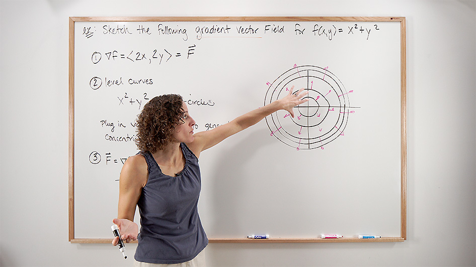
Therefore, if we are given the sphere \(f\left( {x,y,z} \right) = {x^2} + {y^2} + {z^2} – {a^2}\) then the level curves will be circles \(k = {x^2} + {y^2}\) with the gradient vectors \(\nabla f = \left\langle {2x,2y} \right\rangle \) (shown in red) in \({\mathbb{R}^2}\):
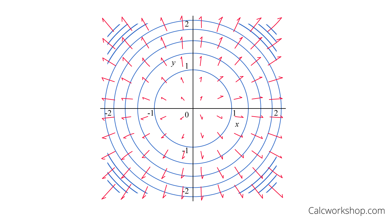
Gradient Vector Field Level Curves
Thus, the gradient vector field \(\nabla f = \left\langle {2x,2y,2z} \right\rangle \) of the sphere \(f\left( {x,y,z} \right) = {x^2} + {y^2} + {z^2} – {a^2}\) in \({\mathbb{R}^3}\) would look something like this:
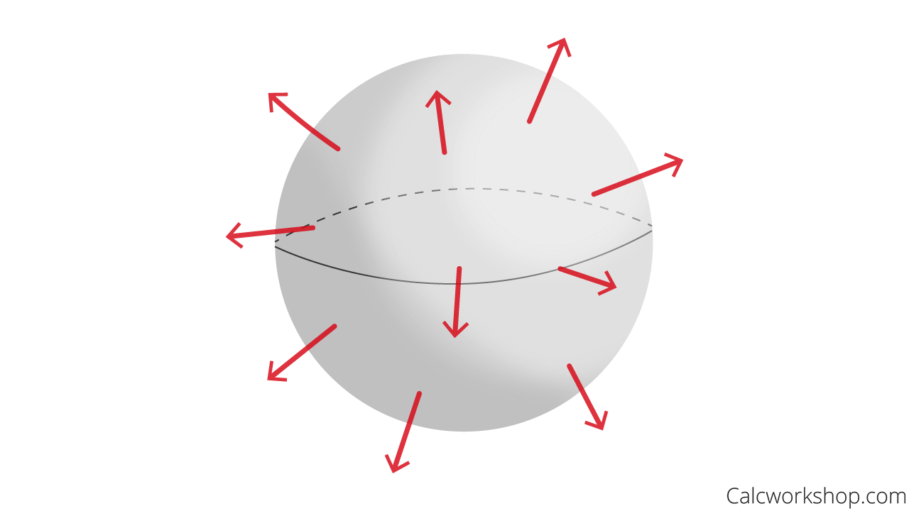
Three Dimensional Gradient Field
Isn’t it awesome to see how our previous learning of gradients helps us understand gradient vector fields!
Conservative Vector Field
But now, this brings us to an important topic as we navigate vector fields.
What are conservative fields?
A vector field \(\overrightarrow F \) is called a conservative vector field if it is the gradient of some scalar function.
In other words, if there exists a function \(f\) such that \(\overrightarrow F = \nabla f\), then \(\overrightarrow F \) is a conservative vector field and \(f\) is a potential function for \(\overrightarrow F \).
Example
Let’s take a look at an example.
Show that \(\overrightarrow F = \nabla f\) if \(\vec{F}=\langle y-3, x+2\rangle\) and \(f\left( {x,y} \right) = xy – 3x + 2y\).
Well, all we have to do is take the partial derivatives of our potential function \(f\) and see if they match the components of \(\overrightarrow F \).
\begin{equation}
f_{x}=y-3 \text { and } f_{y}=x+2 \text { and } \nabla f=\left\langle f_{x}, f_{y}\right\rangle=\langle y-3, x+2\rangle
\end{equation}
\begin{equation}
\vec{F}=\langle y-3, x+2\rangle=\nabla f=\langle y-3, x+2\rangle
\end{equation}
See, all we had to do is verify that the gradient vector for \(f\) is identical to \(\overrightarrow F \).
We will learn more about conservative fields and potential functions in future lessons. Ahh, great things to come.
In fact, everything in this video has far-reaching applications to what we will see in future lessons, such as Line Integrals, Surface Integrals, and more, as vector fields have incredible applications to the patterns we see in our physical world.
So, let’s jump right into our lesson and learn about vector fields!
Video Tutorial w/ Full Lesson & Detailed Examples (Video)
Get access to all the courses and over 450 HD videos with your subscription
Monthly and Yearly Plans Available
Still wondering if CalcWorkshop is right for you?
Take a Tour and find out how a membership can take the struggle out of learning math.
