Quadratic Form
Matrix Approach for Conic Sections

Picture yourself playing a game of Clue, where the objective is to solve a mystery involving quadratic forms and conic sections.

In Clue, players gather evidence and deduce the hidden truth behind the crime by identifying the who, where, and with what weapon.

Similarly, in our quadratic forms investigation, we’ll use linear algebra techniques to reveal the hidden conic sections within the equations by identifying their shape, orientation, and transformation properties.

So grab your detective hat and let’s start our investigation with the matrix representation of quadratic forms.

Matrix Representation of Quadratic Forms

A quadratic form is a function Q defined on \(\mathbb{R}^{n}\) such that \(Q: \mathbb{R}^{n} \rightarrow \mathbb{R}\) that can be written in the form \(Q(x)=x^{T} A x\), where A is a symmetric matrix and is called the matrix of the quadratic form.

But first, we need to make a connection between the quadratic form and its associated symmetric matrix.

When given a quadratic function, we place the coefficient of each squared term down the main diagonal, and half of each cross-product term split symmetrically.

Examples: Finding the Matrix of Quadratic Forms

For example, let’s find the matrix of the quadratic form:

\begin{equation}
\textcolor{red}{a} x_1^2+\textcolor{blue}{b} x_1 x_2+\textcolor{green}{c} x_2^2 \Rightarrow\left[\begin{array}{cc}
\textcolor{red}{a} & \frac{\textcolor{blue}{b}}{2} \\
\frac{\textcolor{blue}{b}}{2} & \textcolor{green}{c}
\end{array}\right]
\end{equation}

\begin{equation}
\textcolor{red}{-5} x_1^2+\textcolor{blue}{8} x_1 x_2+\textcolor{green}{9} x_2^2 \Rightarrow\left[\begin{array}{cc}
\textcolor{red}{-5} & \textcolor{blue}{4} \\
\textcolor{blue}{4} & \textcolor{green}{9}
\end{array}\right]
\end{equation}

\begin{equation}
\textcolor{red}{3} x_1^2+\textcolor{blue}{-4} x_1 x_2+\textcolor{green}{6} x_2^2 \Rightarrow\left[\begin{array}{cc}
\textcolor{red}{3} & \textcolor{blue}{-2} \\
\textcolor{blue}{-2} & \textcolor{green}{6}
\end{array}\right]
\end{equation}

\begin{equation}
\textcolor{black}{8} x_1^2+\textcolor{black}{7} x_2^2+\textcolor{black}{-3} x_3^2+\textcolor{blue}{-6} x_1 x_2+\textcolor{red}{4} x_1 x_3+\textcolor{green}{-2} x_2 x_3 \Rightarrow\left[\begin{array}{ccc}
\textcolor{black}{8} & \textcolor{blue}{-3} & \textcolor{red}{2} \\
\textcolor{blue}{-3} & \textcolor{black}{7} & \textcolor{green}{-1} \\
\textcolor{red}{2} & \textcolor{green}{-1} & \textcolor{black}{-3}
\end{array}\right]
\end{equation}

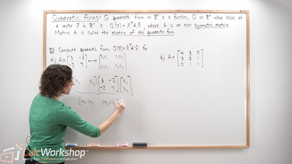
And with this knowledge, we can reverse this process by computing \(x^{T} A x\)

For example, if we are given the symmetric matrix \(\left[\begin{array}{cc}3 & -2 \\ -2 & 7\end{array}\right]\) we can write the quadratic form as follows.

\begin{equation}
x^T A x=\left[\begin{array}{ll}
x_1 & x_2
\end{array}\right]\left[\begin{array}{cc}
3 & -2 \\
-2 & 7
\end{array}\right]\left[\begin{array}{l}
x_1 \\
x_2
\end{array}\right]
\end{equation}

\begin{equation}
\Rightarrow 3 x_1 x_1-2 x_1 x_2-2 x_2 x_1+7 x_2 x_2
\end{equation}

\begin{equation}
\Rightarrow 3 x_1^2-4 x_1 x_2+7 x_2^2
\end{equation}

See, it’s easy. Don’t worry; we’ll work through numerous examples in the video to help make sense of this process.

While this is great, what’s the point?

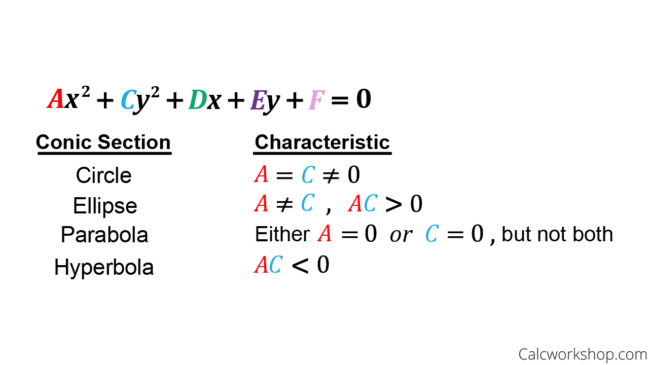
Back in Algebra 2 or Precalculus, we learned about conic sections:

• Parabola
• Circle
• Ellipse
• Hyperbola

But all of the conics we studied could be graphed on the xy-plane as they contained no cross-product terms.

Change of Variables in Quadratic Forms

What do we do if our conic section does have a cross product term? How can we identify it and subsequently graph it?

Ahh, this is why we need matrices and a technique called the change of variable in a quadratic form!

If \(\vec{x}\) represents a variable vector in \(\mathbb{R}^{n}\), then a change of variable is an equation of the form \(\vec{x}=P \vec{y}\) or \(\vec{y}=P^{-1} \vec{x}\)

Where \(\mathrm{P}\) is an invertible matrix that orthogonally diagonalizes matrix \(\mathrm{A}\) and \(\vec{y}\) is a new variable vector in \(\mathbb{R}^{n}\).

Principal Axis Theorem

This leads us directly to the Principal Axis Theorem, which states that if we let A be a square \(n \times n\) matrix, then there is an orthogonal change of variable, \(\vec{x}=\vec{P}\), that transforms the quadratic form \(x^{T} A x\) into a quadratic form \(y^{T} D y\) with no cross-product term. And the columns of \(\mathrm{P}\) are called the principal axes and determine the axis of rotation.

Confused?

Steps for Making a Change of Variables

Don’t fear. Here are the steps for making a change of variables:

1. Make the matrix A of the quadratic form like we did for the examples above.
2. Find eigenvalues by solving the characteristic equation.
3. Identify each eigenspace (i.e., find the eigenvectors that correspond to each eigenvalue)
4. Check for orthogonality, and if necessary, apply the Gram-Schmidt process
5. Normalize to create matrix \(P\) that is orthonormal
6. Write \(P\) and \(D\) matrices and use them to create the transformed quadratic equation without cross-product terms and identify the quadratic form.

Example: Transforming Quadratic Forms

Let’s look at an example.

Transform the quadratic form \(Q(x)=8 x_{1}^{2}+6 x_{1} x_{2}\) into one with no cross-product term.

First, we will find the matrix of the quadratic form like we did for the examples above.

\begin{equation}
Q(x)=8 x_1^2+6 x_1 x_2
\end{equation}

\begin{equation}
\Rightarrow Q(x)=8 x_1^2+6 x_1 x_2+0 x_2^2
\end{equation}

\begin{equation}
\Rightarrow\left[\begin{array}{ll}
8 & 3 \\
3 & 0
\end{array}\right]
\end{equation}

Next, we will find our eigenvalues.

\begin{align*}
\begin{aligned}
& \operatorname{det}\left[\begin{array}{cc}
8-\lambda & 3 \\\\
3 & 0-\lambda
\end{array}\right]=0 \\\\
& (8-\lambda)(0-\lambda)-(3)(3)=0 \\\\
& \lambda^{2}-8 \lambda-9=0 \\\\
& (\lambda-9)(\lambda+1)=0 \\\\
& \lambda=9,-1
\end{aligned}
\end{align*}

Now, we will find the basis for the eigenspace associated with each eigenvector.

\begin{equation}
\lambda=9 \Rightarrow\left[\begin{array}{ccc}
-1 & 3 & 0 \\
3 & -9 & 0
\end{array}\right] \sim\left[\begin{array}{ccc}
1 & -3 & 0 \\
0 & 0 & 0
\end{array}\right]
\end{equation}

\begin{equation}
\Rightarrow \vec{x}=\left[\begin{array}{l}
3 \\
1
\end{array}\right]
\end{equation}

\begin{equation}
\lambda=-1 \Rightarrow\left[\begin{array}{lll}
9 & 3 & 0 \\
3 & 1 & 0
\end{array}\right] \sim\left[\begin{array}{ccc}
1 & 1 / 3 & 0 \\
0 & 0 & 0
\end{array}\right]
\end{equation}

\begin{equation}
\Rightarrow \vec{x}=\left[\begin{array}{c}
-1 / 3 \\
1
\end{array}\right] \text { or } \quad \vec{x}=\left[\begin{array}{c}
-1 \\
3
\end{array}\right]
\end{equation}

Okay, so now that we have our two eigenvectors, we must verify that they are orthogonal.

\begin{align*}
\underbrace{\left[\begin{array}{l}
3 \\
1
\end{array}\right]}_{v_{1}} \underbrace{\left[\begin{array}{c}
-1 \\
3
\end{array}\right]}_{v_{2}} \quad v_{1} \cdot v_{2}=0
\end{align*}

Now, it is time to normalize our vectors to create an orthonormal \(\mathrm{P}\) matrix.

\begin{equation}
\left\|v_1\right\|=\sqrt{(3)^2+(1)^2}=\sqrt{10}
\end{equation}

\begin{equation}
\Rightarrow u_1=\frac{1}{\sqrt{10}}\left[\begin{array}{l}
3 \\
1
\end{array}\right]
\end{equation}

\begin{equation}
=\left[\begin{array}{c}
3 / \sqrt{10} \\
1 / \sqrt{10}
\end{array}\right]
\end{equation}

\begin{equation}
\left\|v_2\right\|=\sqrt{(-1)^2+(3)^2}=\sqrt{10}
\end{equation}

\begin{equation}
\Rightarrow u_2=\frac{1}{\sqrt{10}}\left[\begin{array}{c}
-1 \\
3
\end{array}\right]
\end{equation}

\begin{equation}
=\left[\begin{array}{c}
-1 / \sqrt{10} \\
3 / \sqrt{10}
\end{array}\right]
\end{equation}

\begin{equation}
P=\left[\begin{array}{cc}
3 / \sqrt{10} & -1 / \sqrt{10} \\
1 / \sqrt{10} & 3 / \sqrt{10}
\end{array}\right], \quad D=\left[\begin{array}{cc}
9 & 0 \\
0 & -1
\end{array}\right]
\end{equation}

And remembering that \(A=P D P^{-1}=P D P^{T}\) from our previous lesson on symmetric matrices, we can verify our work as follows, knowing that the columns of \(\mathrm{P}\) are our principal axes.

\begin{align*}
\left[\begin{array}{ll}
8 & 3 \\
3 & 0
\end{array}\right]=\left[\begin{array}{cc}
3 / \sqrt{10} & -1 / \sqrt{10} \\
1 / \sqrt{10} & 3 / \sqrt{10}
\end{array}\right]\left[\begin{array}{cc}
9 & 0 \\
0 & -1
\end{array}\right]\left[\begin{array}{cc}
3 / \sqrt{10} & 1 / \sqrt{10} \\
-1 / \sqrt{10} & 3 / \sqrt{10}
\end{array}\right]
\end{align*}

Lastly, we write our new quadratic form and identify the conic section.

\begin{equation}
x^T A x=y^T D y
\end{equation}

\begin{equation}
\Rightarrow\left[\begin{array}{ll}
y_1 & y_2
\end{array}\right]\left[\begin{array}{cc}
9 & 0 \\
0 & -1
\end{array}\right]\left[\begin{array}{l}
y_1 \\
y_2
\end{array}\right]
\end{equation}

\begin{equation}
=9 y_1 y_1-y_2 y_2 \Rightarrow \underbrace{9 y_1^2-y_2^2}_{\text {Hyperbola }}
\end{equation}

And that’s all we have to do to transform the quadratic form!

Identifying Quadratic Forms

Now, there are some other important properties to know when identifying a quadratic form \(\mathrm{Q}\).

A quadratic form \(\mathrm{Q}\) is:

• Positive definite if \(Q(x)>0\) for all \(\vec{x} \neq \overrightarrow{0}\) (i.e., the eigenvalues of \(\mathrm{A}\) are all positive)
• Negative definite if \(Q(x)<0\) for all \(\vec{x} \neq \overrightarrow{0}\) (i.e., the eigenvalues of \(\mathrm{A}\) are all negative)
• Indefinite if \(Q(x)\) assumes both positive and negative values. (i.e., the eigenvalues of \(\mathrm{A}\) are both positive and negative)

If \(\lambda_{1} \cdot \lambda_{2}>0\), then the quadratic form after the change of variables will be an ellipse or a circle.

If \(\lambda_{1} \cdot \lambda_{2}<0\), then the quadratic form after the change of variables will be a hyperbola.

If only one \(\lambda\), then the quadratic form after the change of variables will be a parabola.

Next Steps

There’s a lot to unpack in this lesson. You’ll work through examples step-by-step as you learn how to:

• Compute the quadratic form
• Find the matrix for the quadratic form
• Classify the quadratic form
• Use a change of variables to eliminate cross-product terms

Let’s get started!

Video Tutorial w/ Full Lesson & Detailed Examples

Get access to all the courses and over 450 HD videos with your subscription

Monthly and Yearly Plans Available

Get My Subscription Now

Still wondering if CalcWorkshop is right for you?
Take a Tour and find out how a membership can take the struggle out of learning math.