Diagonalization of Symmetric Matrices
Steps & Strategies

Have you ever wondered how to simplify and understand complex mathematical structures like symmetric matrices?

Diagonalization of symmetric matrices is like solving a Rubik’s Cube, where each twist and turn brings you closer to the neatly organized and aligned colors.

By breaking down the complexities of symmetric matrices into more manageable components, we can extract valuable insights and solve problems more efficiently.

So, let’s jump in and solve this puzzle one step at a time.

Introduction to Symmetric Matrices

Ready? First, let’s understand the basics.

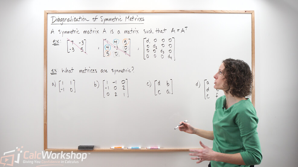
If a square matrix \(\mathrm{A}\) equals its transpose, it is considered a symmetric matrix.

This means that the main diagonal entries are arbitrary values, but its other entries occur in pairs on either side of the main diagonal.

For example, the following \(3 \times 3\) matrix shows arbitrary values down the main diagonal in black, but the pairs of entries on either side are shown in red, blue, and green. Such a matrix is considered symmetric.

\begin{equation}
\left[\begin{array}{lll}
\color{black}{a} & \color{red}{b} & \color{blue}{c} \\\
\color{red}{b} & \color{black}{d} & \color{green}{e} \\\
\color{blue}{c} & \color{green}{e} & \color{black}{f}
\end{array}\right]
\end{equation}

As you can see, \(A=A^{T}\), thus making it symmetric.

And if you’ve ever studied graph theory or taken discrete mathematics, you may recognize that a symmetric matrix is sometimes called an incident matrix.

Besides a symmetric matrix being “symmetric,” what’s so special about it?

Properties of Symmetric Matrices

Let’s look at a few properties related to symmetric matrices:

1. The product of any matrix and its transpose is symmetric. That is, both \(A A^{T}\) and \(A^{T} A\) are symmetric matrices.
2. If \(\mathrm{A}\) is any square matrix, then \(A+A^{T}\) is symmetric.
3. The sum of two symmetric matrices is also symmetric.
4. Eigenvectors corresponding to distinct eigenvalues are orthogonal.

Diagonalization of Symmetric Matrices

And it’s this last property that gives us two compelling theorems regarding the diagonalization of symmetric matrices:

1. If \(\mathrm{A}\) is a symmetric matrix, then any two eigenvectors from different eigenspaces are orthogonal.
2. Additionally, an \(n \times n\) matrix A is orthogonally diagonalizable if and only if \(\mathrm{A}\) is a symmetric matrix.

Now, that’s pretty special! Because if we have a symmetric matrix, we can quickly determine that it’s diagonalizable.

Orthogonal Diagonalization Example

Let’s look at an example where we will orthogonally diagonalize a symmetric matrix and give an orthogonal matrix \(\mathrm{P}\) and diagonal matrix \(\mathrm{D}\) if

\begin{align*}
A=\left[\begin{array}{ccc}
7 & -4 & 4 \\
-4 & 5 & 0 \\
4 & 0 & 9
\end{array}\right]
\end{align*}

First, we will find our characteristic polynomial and solve the equation to find our eigenvalues.

\begin{align*}
\begin{aligned}
& \operatorname{det}\left[\begin{array}{ccc}
7-\lambda & -4 & 4 \\
-4 & 5-\lambda & 0 \\
4 & 0 & 9-\lambda
\end{array}\right]=0 \\\\
& -\lambda^{3}+21 \lambda^{2}-111 \lambda+91=0 \\\\
& -(\lambda-13)(\lambda-7)(\lambda-1)=0 \\\\
& \lambda=13,7,1
\end{aligned}
\end{align*}

Because we have three distinct eigenvalues, and matrix \(\mathrm{A}\) is symmetric, we are guaranteed distinct eigenvectors. So, now it’s time to find them.

If

\begin{equation}
\lambda=13 \Rightarrow\left[\begin{array}{cccc}
-6 & -4 & 4 & 0 \\
-4 & -8 & 0 & 0 \\
4 & 0 & -4 & 0
\end{array}\right] \sim\left[\begin{array}{cccc}
1 & 0 & -1 & 0 \\
0 & 1 & 1 / 2 & 0 \\
0 & 0 & 0 & 0
\end{array}\right]
\end{equation}

\begin{equation}
\Rightarrow \vec{x}=\left[\begin{array}{c}
1 \\
-1 / 2 \\
1
\end{array}\right] \text { or } \quad \vec{x}=\left[\begin{array}{c}
2 \\
-1 \\
2
\end{array}\right]
\end{equation}

\begin{equation}
\lambda=7 \Rightarrow\left[\begin{array}{cccc}
0 & -4 & 4 & 0 \\
-4 & -2 & 0 & 0 \\
4 & 0 & 2 & 0
\end{array}\right] \sim\left[\begin{array}{cccc}
1 & 0 & 1 / 2 & 0 \\
0 & 1 & -1 & 0 \\
0 & 0 & 0 & 0
\end{array}\right]
\end{equation}

\begin{equation}
\Rightarrow \vec{x}=\left[\begin{array}{c}
-1 / 2 \\
1 \\
1
\end{array}\right] \text { or } \vec{x}=\left[\begin{array}{c}
-1 \\
2 \\
2
\end{array}\right]
\end{equation}

\begin{equation}
\lambda=1 \Rightarrow\left[\begin{array}{cccc}
6 & -4 & 4 & 0 \\
-4 & 4 & 0 & 0 \\
4 & 0 & 8 & 0
\end{array}\right] \sim\left[\begin{array}{llll}
1 & 0 & 2 & 0 \\
0 & 1 & 2 & 0 \\
0 & 0 & 0 & 0
\end{array}\right]
\end{equation}

\begin{equation}
\Rightarrow \vec{x}=\left[\begin{array}{c}
-2 \\
-2 \\
1
\end{array}\right]
\end{equation}

Therefore, our eigenspace is

\begin{align*}
\left\{\left[\begin{array}{c}
2 \\
-1 \\
2
\end{array}\right],\left[\begin{array}{c}
-1 \\
2 \\
2
\end{array}\right],\left[\begin{array}{c}
-2 \\
-2 \\
1
\end{array}\right]\right\}
\end{align*}

Now we have to ensure that each pair of vectors are orthogonal.

\begin{equation}
\underbrace{\left[\begin{array}{c}
2 \\
-1 \\
2
\end{array}\right]}_{v_1}, \underbrace{\left[\begin{array}{c}
-1 \\
2 \\
2
\end{array}\right]}_{v_2}, \underbrace{\left[\begin{array}{c}
-2 \\
-2 \\
1
\end{array}\right]}_{v_3}
\end{equation}

\begin{equation}
v_1 \cdot v_2=0 \text { and } v_1 \cdot v_3=0 \text { and } v_2 \cdot v_3=0
\end{equation}

Now that we have shown that our eigenspace is orthogonal, we must normalize each vector to create our orthonormal P matrix.

\begin{equation}
\left\|v_1\right\|=\sqrt{(2)^2+(-1)^2+(2)^2}
\end{equation}

\begin{equation}
=\sqrt{9}=3
\end{equation}

\begin{equation}
\Rightarrow u_1=\frac{1}{3}\left[\begin{array}{c}
2 \\
-1 \\
2
\end{array}\right]=\left[\begin{array}{c}
2 / 3 \\
-1 / 3 \\
2 / 3
\end{array}\right]
\end{equation}

\begin{equation}
\left\|v_2\right\|=\sqrt{(-1)^2+(2)^2+(2)^2}
\end{equation}

\begin{equation}
=\sqrt{9}=3
\end{equation}

\begin{equation}
\Rightarrow u_2=\frac{1}{3}\left[\begin{array}{c}
2 \\
-1 \\
2
\end{array}\right]=\left[\begin{array}{c}
-1 / 3 \\
2 / 3 \\
2 / 3
\end{array}\right]
\end{equation}

\begin{equation}
\left\|v_3\right\|=\sqrt{(-2)^2+(-2)^2+(1)^2}
\end{equation}

\begin{equation}
=\sqrt{9}=3
\end{equation}

\begin{equation}
\Rightarrow u_2=\frac{1}{3}\left[\begin{array}{c}
-2 \\
-2 \\
1
\end{array}\right]=\left[\begin{array}{c}
-2 / 3 \\
-2 / 3 \\
1 / 3
\end{array}\right]
\end{equation}

Thus, our P matrix, which consists of normalized eigenvectors, and our D matrix, which is the diagonal matrix representing the eigenvalues, is as follows:

\begin{align*}
P=\left[\begin{array}{ccc}
2 / 3 & -1 / 3 & -2 / 3 \\
-1 / 3 & 2 / 3 & -2 / 3 \\
2 / 3 & 2 / 3 & 1 / 3
\end{array}\right], \quad D=\left[\begin{array}{ccc}
13 & 0 & 0 \\
0 & 7 & 0 \\
0 & 0 & 1
\end{array}\right]
\end{align*}

And we can verify the accuracy of our answer by showing \(A=P D P^{-1}\).

\begin{align*}
\left[\begin{array}{ccc}
7 & -4 & 4 \\
-4 & 5 & 0 \\
4 & 0 & 9
\end{array}\right]=\left[\begin{array}{ccc}
2 / 3 & -1 / 3 & -2 / 3 \\
-1 / 3 & 2 / 3 & -2 / 3 \\
2 / 3 & 2 / 3 & 1 / 3
\end{array}\right]\left[\begin{array}{ccc}
13 & 0 & 0 \\
0 & 7 & 0 \\
0 & 0 & 1
\end{array}\right]\left[\begin{array}{ccc}
2 / 3 & -1 / 3 & -2 / 3 \\
-1 / 3 & 2 / 3 & 2 / 3 \\
-2 / 3 & -2 / 3 & 1 / 3
\end{array}\right]
\end{align*}

But here’s something very interesting …Look at the two matrices \(P\) and \(P^{-1}\). They are just the transpose of each other!

This is incredible because if matrix \(\mathrm{A}\) is orthogonally diagonalizable, as we have just shown, then \(A=P D P^{T}=P D P^{-1}\)

Cool!

Next Steps

Together, you will:

• Learn to identify symmetric matrices and determine how to use them for identifying conic sections with cross product terms, where two variables are being multiplied together, such as “xy.”
• Discover that to identify the conic section without looking at the graph, you need to analyze the function’s eigenvalues and eigenvectors in order to rotate the conic to a new set of axes – an orthogonal set!
• Explore several theorems and definitions, and review the Gram-Schmidt process to understand the steps needed to diagonalize a symmetric matrix.
• Delve into the Spectral Theorem for Symmetric Matrices and Spectral Decomposition.

Let’s dive in and get started!

Video Tutorial w/ Full Lesson & Detailed Examples

Get access to all the courses and over 450 HD videos with your subscription

Monthly and Yearly Plans Available

Get My Subscription Now

Still wondering if CalcWorkshop is right for you?
Take a Tour and find out how a membership can take the struggle out of learning math.