Did you know that our ability to understand the relationships among quantities that vary can be modeled using something called Least-Squares Lines?

Jenn, Founder Calcworkshop®, 15+ Years Experience (Licensed & Certified Teacher)
In fact, a least-squares line can be used to predict future values, which can be pretty useful in science, business, and engineering.
Finding the Linear Regression Line
Okay, so what is the least-squares regression line (LSRL)?
It is a line that “best fits” the data, which is why least-squares regression is sometimes called the line of best fit.
Suffice it to say the simplest relationship between two variables is a line, and a least-square regression line matches the pattern or relationship of a set of paired data as closely as possible.
Therefore, if a straight-line relationship is observed, we can describe this association with a regression line. This trend line minimizes the prediction of error, called residuals, as discussed by Shafer and Zhang.
Regression Equation
And the regression equation provides a rule for predicting or estimating the response variable’s values when the two variables are linearly related.

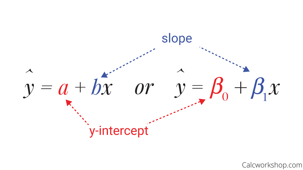
Least Squares Regression Line Equation
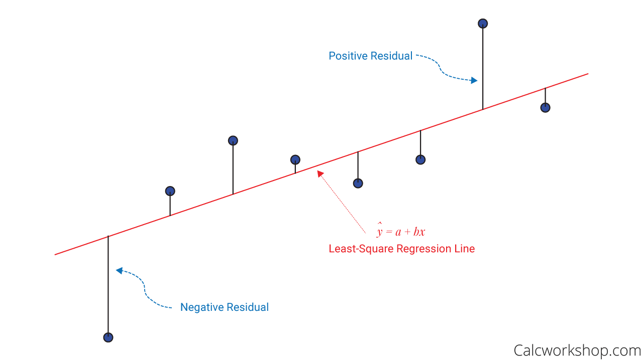
Residuals
Wait! What are residuals?
Residuals are the differences between the observed and predicted values. It measures the distance from the regression line (predicted value) and the actual observed value. In other words, it helps us to measure error, or how well our least-squares line “fits” our data.

Residual Plot Interpretation
Okay, so knowing that we are looking for an equation of the form.
How do we find the y-intercept
Computing the Least-Squares Solution
By computing the least-squares solution of
Remember how in our previous lesson we learned that the least squares solution of the inconsistent matrix equation
Well, the same thing is happening here.
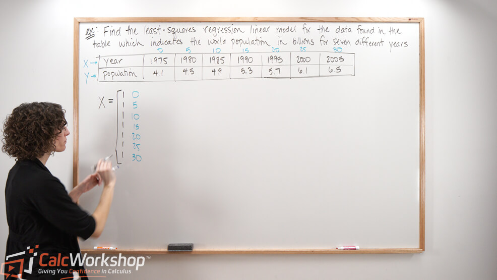
Constructing the Design Matrix and Observation Vector
Therefore,
Working Through an Example
Let’s look at an example to get a feel for how this works.
Find the equation
Step 1: Creating the Design Matrix
First, we will create our Design Matrix. Noticing that there are four data points, we will have a
Step 2: Forming the Observation Vector
Next, we will create our Observation vector, a column matrix consisting of the
Step 3: Performing Matrix Multiplication
Now we will compute our matrix multiplication to find
Step 4: Determining the Least-Squares Line
And lastly, we will find our least squares solution by row reducing our augmented matrix.
Finally, we can write our least-square line as follows:
Awesome!
Expanding to Regression Curves
And here’s the exciting part – we aren’t limited to just regression lines, we can also create regression curves!
Quadratic Regression
Yep, we can use the process of least-square to fit parabolic curves, cubic curves, and more.
Quadratics:
Cubic Regression
Cubics:
Next Steps
Don’t worry. We’ll work through numerous examples together and learn how to find least-squares lines and curves given data values and use our regression to predict future values.
Let’s jump on in!
Video Tutorial w/ Full Lesson & Detailed Examples

Get access to all the courses and over 450 HD videos with your subscription
Monthly and Yearly Plans Available
Still wondering if CalcWorkshop is right for you?
Take a Tour and find out how a membership can take the struggle out of learning math.