What is a double integral?

Jenn, Founder Calcworkshop®, 15+ Years Experience (Licensed & Certified Teacher)
For starters, it’s the path to calculate the volume of a region in three-space.
Definite Integral Review
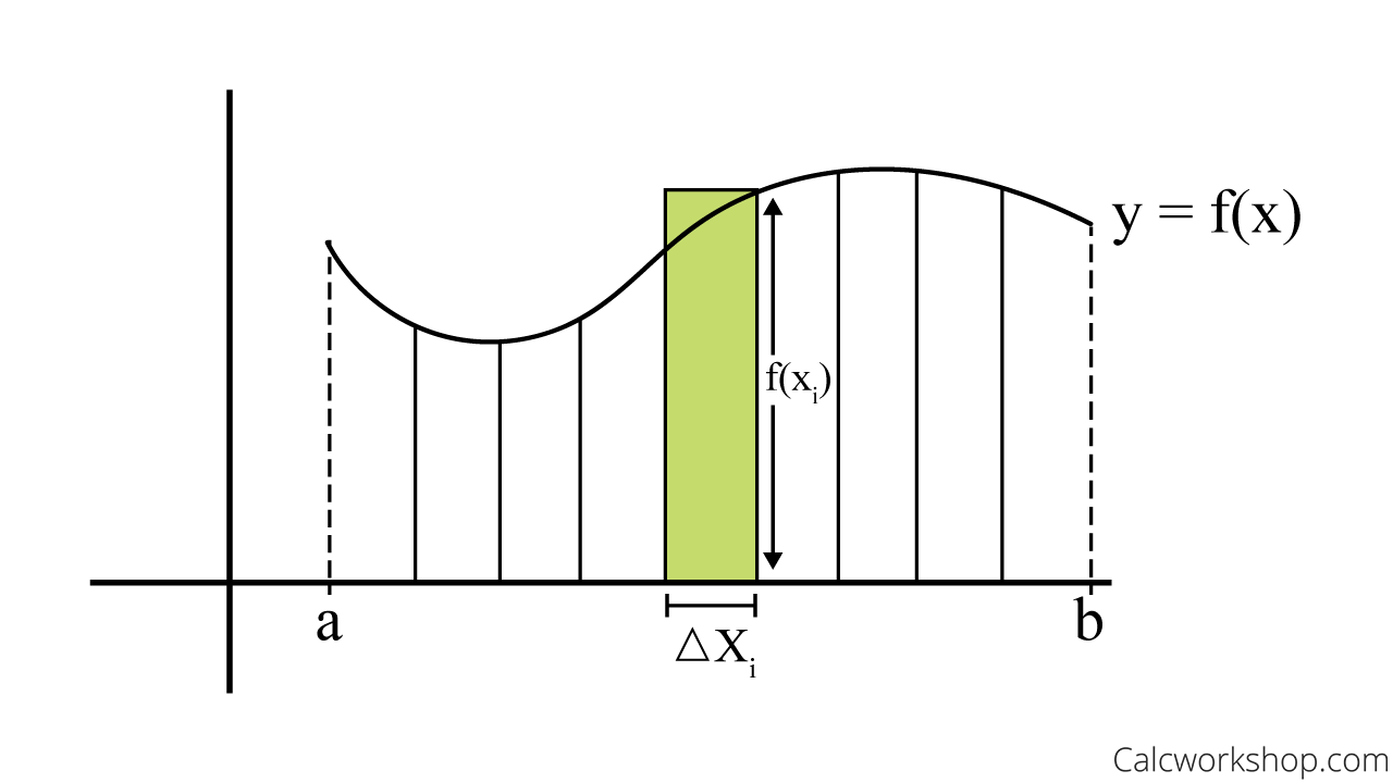
Recall how in single variable calculus we learned how to subdivide the area of a region into simple geometric shapes, namely rectangles.
By summing the area of each of these subdivided rectangles we were able to estimate the overall area of the plane region.

Estimating Area Under A Curve – Riemann Sum
This discovery led us to the notion of antidifferentiation, namely the definite integral. Noticing how a region can be bounded and “sliced” horizontally or vertically allowed us to integrate the area between two curves quickly and easily.
So, if we can find the area of a region by dividing the area into rectangular strips, we can use a similar approach for finding volume of a region in three-dimensions.
Let’s see how.
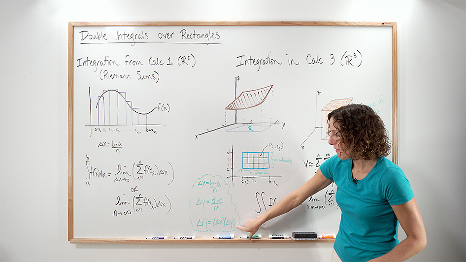
Double Integrals Over Rectangles
Since we are dealing with a three-dimensional object, we will begin by dividing the region into small rectangular prisms and add up the volumes of all of those boxes to approximate the overall volume.

Evaluating Volume (Rectangular Prisms)
And intuition tells us that if we take the limit as both

Sample Point In Rectangular Region
This process for evaluating the volume of a surface down to the plane is known as double integrals over rectangles.
Therefore, if we let
exists, then
Example
Let’s look at an example to see how this works.
Suppose
Approximate
To begin we superimposing a rectangular grid over the xy-plane and subdivide this grid into rectangles in both the x- and y- direction using the dimensions of our region
and find our value, knowing that:
Subdivide Rectangular Grid
Next, we will find the center of each square, as these will be our nine sample points. We do this by taking the average for both the
and distances within each rectangle.
Midpoint Rule Sample Points
Finally, we will substitute our nine sample points into our function formula to find the volume of the surface knowing that volume is the product of the height and the area of the base.
We just found the volume under the surface! Not bad, right?
It’s just like Riemann sums from calculus 1.
Together in our lesson we will learn how to calculate double integrals over rectangles to find the volume of a surface by identifying sample points, such as lower or upper corners of each subrectangle, and calculating the areas using the double Riemann sum approximation and the midpoint rule for double integrals.
It’s going to be a fun trip down memory lane as we recall our integration approximations from single-variable calculus and learn how to apply our skills to find volume for functions of several variables.
Let’s jump right in.
Video Tutorial w/ Full Lesson & Detailed Examples (Video)

Get access to all the courses and over 450 HD videos with your subscription
Monthly and Yearly Plans Available
Still wondering if CalcWorkshop is right for you?
Take a Tour and find out how a membership can take the struggle out of learning math.

