Matrix Operations (Essential Techniques Explained)

Did you know that matrices are used in nearly every branch of mathematics?

Jenn (B.S., M.Ed.) of Calcworkshop® teaching matrix operations

Jenn, Founder Calcworkshop^®, 15+ Years Experience (Licensed & Certified Teacher)

And our ability to solve and analyze linear systems of equations is greatly enhanced when we can perform algebraic operations with matrices.

What type of operations?

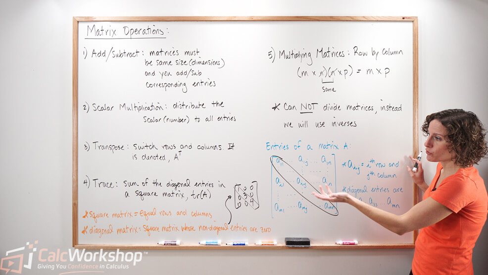
Addition, subtraction, multiplication of matrices, the transpose and trace, as well as how to calculate the determinant of a matrix.

Understanding Special Matrices

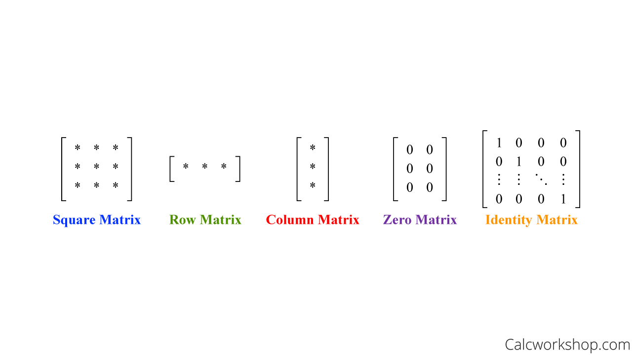
But before we can jump into the basic matrix operations, we need to review some special matrices: square matrix, row matrix, column matrix, zero matrix, and identity matrix, as they will be required in understanding some critical matrix properties.

A square matrix is an $n \times n$ matrix where the number of rows equals the number of columns. A row matrix is a $1 \times n$ matrix such that there is only one row with $n$ columns. A column matrix is a $n \times 1$ array with $n$ rows and only one column. A matrix containing only zero elements is called a zero matrix, denoted $\vec{0}$ . And the identity matrix is a square matrix such that the elements along the main diagonal are all $1 s$ and the rest are $0 s$ .

Properties – Special Matrices

Basic Matrix Operations

Alright, now let’s jump into those fundamental operations.

Throughout our work with matrices so far, we know that we can multiply a matrix by a scalar (number), similar to how we apply the distributive property with parentheses. While the matrix size is not vital for scalar multiplication, it is critical for adding and subtracting matrices.

To add or subtract two matrices, we add or subtract the corresponding element. But there is a warning-only matrices of the same size can be added or subtracted. It is also important to note that when subtracting matrices, what we are really doing is adding the opposite.

$\begin{array}{r} A - B = A + (- B) \end{array}$

Here’s the updated section with the equations formatted according to your specified format, broken up for better display on a narrow page:

For example, let’s find the scalar multiplication, sum, or difference for the following matrices.

$\begin{aligned} 3 [\begin{array}{cc} 5 & - 6 \\ 8 & 9 \end{array}] & = [\begin{array}{cc} 3 \cdot 5 & 3 \cdot (- 6) \\ 3 \cdot 8 & 3 \cdot 9 \end{array}] \\ = [\begin{array}{cc} 15 & - 18 \\ 24 & 27 \end{array}] \end{aligned}$

$\begin{aligned} [\begin{array}{cc} 5 & - 6 \\ 8 & 9 \end{array}] + [\begin{array}{cc} - 4 & 6 \\ 8 & - 3 \end{array}] & = [\begin{array}{cc} 5 + (- 4) & - 6 + 6 \\ 8 + 8 & 9 + (- 3) \end{array}] \\ = [\begin{array}{cc} 1 & 0 \\ 16 & 6 \end{array}] \end{aligned}$

$\begin{aligned} [\begin{array}{cc} 5 & - 6 \\ 8 & 9 \end{array}] - [\begin{array}{cc} - 4 & 6 \\ 8 & - 3 \end{array}] & = [\begin{array}{cc} 5 & - 6 \\ 8 & 9 \end{array}] + [\begin{array}{cc} - (- 4) & - (6) \\ - (8) & - (- 3) \end{array}] \\ = [\begin{array}{cc} 5 & - 6 \\ 8 & 9 \end{array}] + [\begin{array}{cc} 4 & - 6 \\ - 8 & 3 \end{array}] \\ = [\begin{array}{cc} 9 & - 12 \\ 0 & 12 \end{array}] \end{aligned}$

Easy, right?

And matrix addition satisfies the closure, commutative, associative, identity, and inverse properties from Algebra!

Matrix Multiplication Explained

Alright, now it’s time to talk about matrix multiplication.

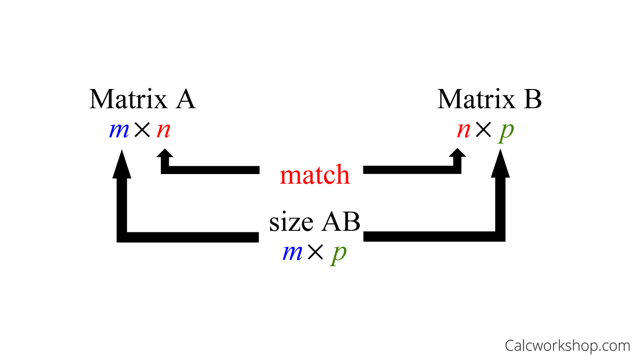
If the number of columns of an $m \times n$ matrix $A$ is the same as the number of rows of an $n \times p$ matrix B, then the product matrix $A B$ is found as $a_{i 1} b_{1 j} + a_{i 2} b_{2 j} + \dots + a_{i n} b_{n j}$ creating an $m \times p$ matrix.

Huh?

It’s really not so hard.

First, we must determine the dimensions of the product matrix and then multiply row by column.

Matrix Multiplication Composition

Here’s the updated section with the equations formatted according to your specified format, broken up for better display on a narrow page:

It’s best to see this rule in action with an example.

Find the product $A B$ if $A = [\begin{array}{ccc} - 3 & 4 & 2 \\ 5 & 0 & 4 \end{array}]$ and $B = [\begin{array}{cc} - 6 & 4 \\ 2 & 3 \\ 3 & - 2 \end{array}]$

First, we confirm the size of the product matrix:

$\begin{aligned} A & = 2 \times 3 \\ B & = 3 \times 2 \\ A B & = 2 \times 2 \end{aligned}$

Then we multiply corresponding elements from the rows of $A$ and the columns of $B$ and calculate the sum of the products:

$\begin{aligned} [\begin{array}{ccc} - 3 & 4 & 2 \\ 5 & 0 & 4 \end{array}] [\begin{array}{cc} - 6 & 4 \\ 2 & 3 \\ 3 & - 2 \end{array}] & = [\begin{array}{cc} (- 3) \cdot (- 6) + 4 \cdot 2 + 2 \cdot 3 & (- 3) \cdot 4 + 4 \cdot 3 + 2 \cdot (- 2) \\ 5 \cdot (- 6) + 0 \cdot 2 + 4 \cdot 3 & 5 \cdot 4 + 0 \cdot 3 + 4 \cdot (- 2) \end{array}] \\ = [\begin{array}{cc} 32 & - 4 \\ - 18 & 12 \end{array}] \end{aligned}$

Don’t worry! We will work through numerous examples of how to multiply two matrices so you get the hang of it, and we will also look at how to calculate the Powers of a Matrix too.

Now, it is imperative to note that while the associative and distributive properties are satisfied with matrix multiplication, the commutative property is not.

Properties of Matrix Multiplication:

$\begin{aligned} (A B) C & = A (B C) \\ A (B + C) & = A B + A C \\ (B + C) A & = B A + C A \end{aligned}$

Meaning $A B$ does not guarantee that $B A$ . Order matters!

Transpose and Trace of a Matrix

Okay, so now let’s talk about the transpose of a matrix and the trace of a matrix.

The transpose of a matrix is found by switching its rows and columns. In essence, it is the flipped version of the original matrix and is denoted $A^{T}$

If $A = [\begin{array}{cc} 5 & 1 \\ 0 & 2 \\ - 3 & 4 \end{array}]$ then

$\begin{aligned} A^{T} & = [\begin{array}{ccc} 5 & 0 & - 3 \\ 1 & 2 & 4 \end{array}] \end{aligned}$

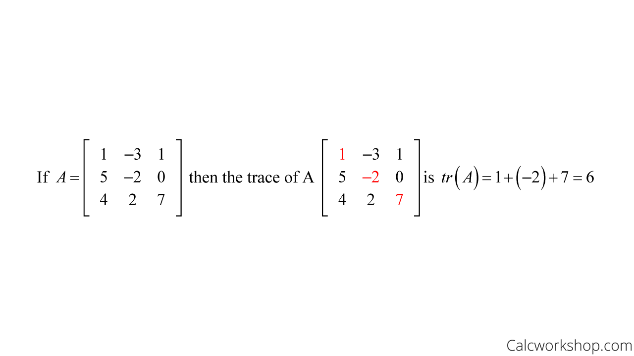
The transpose of a matrix is essential to understanding inverses, estimating variances, transformations, rank, and so much more. Additionally, if $A$ and $B$ are matrices whose sizes are appropriate for the sum and product, then

$\begin{aligned} {(A^{T})}^{T} & = A \\ (A + B)^{T} & = A^{T} + B^{T} \\ (c A)^{T} & = c A^{T}, for some scalar c \\ (A B)^{T} & = B^{T} A^{T} \end{aligned}$

The trace of the matrix is the sum of the main diagonal entries of a square matrix. It allows us to weigh and quantify complexity and is used in mapping, eigenvalues, and vector spaces.

Calculate Trace Square Matrix (Example)

Remember, the trace can only be calculated for square matrices!

Determinant of a Matrix

Finally, we will learn about the determinant.

A determinant is a special number that can be calculated from a square matrix, nicely stated by Math is Fun. In fact, every $n \times n$ matrix $A$ is associated with a real number called the determinant of $A$ , written $\det (A)$ or $| A |$ , that is used in solving systems of equations, finding angles between vectors, vector cross products in calculus, and many other vector operations.

First, we will learn how to calculate a determinant for a $2 \times 2$ matrix, using the following formula: If $A = [\begin{array}{ll} a & b \\ c & d \end{array}]$ then

$\begin{aligned} \det (A) & = | A | \\ = a d - b c \end{aligned}$

For example, if $A = [\begin{array}{cc} 8 & 6 \\ 4 & - 3 \end{array}]$ then

$\begin{aligned} \det (A) & = | A | \\ = 8 \cdot (- 3) - 6 \cdot 4 \\ = - 48 \end{aligned}$

And in the video lesson, we will discover how to apply this rule for a $3 \times 3$ matrix, where we will use a technique called Expansion by Minor (Cofactors) and the array of signs.

Knowing how to calculate a determinant of a matrix will be imperative to our understanding of how to solve systems of equations as well as the Invertible Matrix Theorem, which we will learn in a future lesson.

This lesson packs a punch and will set us off for all future lessons dealing with matrix operations.

Let’s jump right in!

Video Tutorial w/ Full Lesson & Detailed Examples

matrix-operations-and-determinants-example

Get access to all the courses and over 450 HD videos with your subscription

Monthly and Yearly Plans Available

Get My Subscription Now

Still wondering if CalcWorkshop is right for you?
Take a Tour and find out how a membership can take the struggle out of learning math.

4.9 / 5

1,128 Reviews

Kevin S.10-30-24 - CO, United States

I had never even heard of discrete math before I had to take it for my Bachelor's in Cybersecurity. I had actually hoped that my math days were done! I suffered through class not understanding any of the presentations until I stumbled across Calcworkshop. I used the Calcworkshop lessons more than I used my instructor's lectures and my book. I ended up with a high B (just 12 points away from an A) thanks to Jenn. Without her easy to understand style of teaching, I'm not sure I would have even passed the class. Thank you so much!!!

Richard10-29-24 - Norway

Very well structured and site. It is well structured giving a good overview of the different topics regarding all mathematics where you easily can choose which path is applicable to your specific needs.The video lectures are superb with introduction to the topic followed by a detailed theoretically explaination and what I personally get most out of is; heaps of examples where you are taken and shown, step by step, the prosess of solving the problem. They also includd practice sheets and solutions to test yourself after each chapter. There is a lot to undertake on this site, but it provides an easy and understandable interface to map out what you need to do. The site has been very helpfull for me and I highly recommend it.

RobWP10-26-24 - United States

I am taking this course for mainly linear algebra review. It is a course that I have had but fairly long ago. I'm currently working in masters in data science and linear algebra namely transformations is something that has come up and I thought I need a good review on. I so far what I have liked about the course is, the common sense approach. Her approach makes it easy to remember the concepts because of her common sense approach. I like the fact that she gives information that is not really in any textbooks. I can vouch for that because not only have I used textbook recently to review I have had a formal class in the past that used textbooks. She goes over things thoroughly and for the price it's very much worth it. I have had many quarters of formal calculus and differential equations courses and I am kind of anxious to look to see what her approach to calculus is. I can't really answer how this class would be for a novice or someone who has not had linear algebra the past, but I really don't think they need to worry about that. Her method I feel will make a novice be successful and to understand the material. She is very easy to understand. Gives good examples but doesn't beat a dead horse either. What I like about her introductory remarks is that she says what linear algebra is all about and she points out what the core of the linear algebra is about and what you need to know. Having taken it before I would have to agree and she is dead on spot.

Robbin03-18-25 - CO, United States

Very well organized, helpful and comprehensive. It is great also to have access to prior course material so you can easily go back and refresh if you need to. Jenn is very clear and the number of examples leaves one comfortable with each topic. Couldn't be happier.

RCJK03-07-25 - ID, United States

I had to take Calculus I and II as accelerated classes while working full time. It was my first time taking this courses and was very overwhelming. Calcworkshop really made learning the subjects easier for me by having all the subjects easy to find and easy to understand explanations. I received a B in both classes which I am extremely happy with doing the classes in double time.

Jacqueline S.03-07-25 - SC, United States

Jenn is awesome!Her breakdown of the topic is beyond what you would expect. She is showing you how to arrive at the answer instead of doing a simple equation. Most people need to know the why it give confidence and structure to the learning process. This is what Jenn is great at, she knows how to deliver the information to a non math mind in a way that instills knowledge that you can forever draw from as you move forward. It's really well thought out. She is a true master teacher. Thanks for all that you do for us! Hugs n Blessings... JS

Rose M.03-07-25 - CA, United States

Best instructor ever, I have never had Math explained in a way that was so interesting. Her lectures and instruction is explained perfectly, and I will continue to use this for all my future math courses.

A Reviewer03-07-25 - United States

I needed help with college precalculus, they provided more than enough help that allowed me to succeed and get the scores I needed.

Jujuana03-05-25 - MO, United States

I love the videos the way each lesson is explained step by step. I love that she has examples that you can go over again and again in order to understand the way algebra works. I was lost because my instructor was flying through each lesson and I was totally lost. I attached my syllabus and they helped me stay focus on what I was working and give me a guide to go back and refresh what I went over in class.

Stacey01-31-25 - AZ, United States

Hello, I highly recommend getting a subscription to Jenn and her Calcworkshop teaching math service. I did a general, "go from bad to good at math", Google search and found out about Calcworkshop through responses to the topic on reddit. I've just started watching her videos and found them to be extremely helpful. I'm going back to college after a long absence and math was never my strong suit. So I'm starting at the very bottom of her available subjects and going from there. Just watching a couple of the videos has taken me from being dragged along not understanding to following along just fine in my math class. I'm moving from the "I'll never get this", to the "I look forward to understanding this", mindset in approaching math. This for me is huge, and even though I have a long way to go, I'm confident I will get there thanks to Jenn. Totally worth it!

Kathy W.01-14-25 - WA, United States

Calcworkshop is an outstanding source to learn math and understanding math concepts. Jenn is an outstanding master teacher. Every lesson is clearly presented making understanding easy to grasp. Practice lessons with accompanying answers are given for each section. I am 82, a retired teacher and lifelong learner. Learning calculus has always been on my bucket list. Calcworkshop is helping me reach my goal.

Cheryl01-14-25 - NY, United States

Calc workshop is the absolutely best resource for math and I have seen almost everything that exists out there. I have even recommended it to my daughter's school so that all the kids could use the videos during the summer months for the subject they plan to study in the fall. They are guaranteed to get a A if they have watched the videos and completed the problems before taking the class. Students who are weak in areas can access lower level classes and those who seek to advance above grade level can do so. The videos and exercises are crystal clear and the excellent presentations raise the bar for teachers everywhere. I have always believed that one great math teacher is important in the education process. The videos, exercises and problems are excellent. It is not possible to have ANY knowledge gaps. I have never seen anything on the market that even begins to compete with it!

Justin N.12-22-24 - OK, United States

Calculus can be a scary subject. I know I was scared. I had been out of any math class for over 23 years. I had taken an 8 week Calculus 1 class and felt like I was overloaded. Going into Calculus 2 I found CALCWORKSHOP.com. I used the training videos and material to really dive back into Calc 1 and prepare for Calc 2. Long story short with the material provided and ample study time, I finished Calc 2 with a 95%. Thanks Jenn!

Shelby12-10-24 - OH, United States

CalcWorkshop was a wonderful resource as someone going onto a college calculus 1 class after not having taken a math course in a year! Jenn always explained things in a logical order that built upon previous lessons, and the way she explained topics was always easy to understand. Calcworkshop saved this semester for me, and I couldn't be more grateful to have found this site. :)

Jordan Q.12-09-24 - AR, United States

Anyone struggling with math at any level would greatly benefit from this product. I signed up for it immediately after getting a D on my first exam in calculus 2 and ended up getting A's and B's on the remaining exams, getting a B overall in the class. Jenn breaks down the topics, without skipping any steps, in a way that makes them very easy to understand. I highly recommend this product!

N8Booker11-28-24 - MA, United States

I'm in school to get my degree Networking and Cybersecurity and I'm in my first year. I've been away from school for quite a long time so the concepts that are being taught although not foreign to me, have so much dust on them from a lack of being used in real world applications regularly.I stumbled upon CalcWorkshop by pure chance and it has been a game changer for me. Jen filled in the gaps in between what my Professor is teaching at a rapid fire pace and where my brain grasps and applies it. If not for Jen's approach, I'd have failed my test I took miserably!Am I grateful? It goes beyond words and not I recommend her workshops to everyone!

Kevin S.10-30-24 - CO, United States

Richard10-29-24 - Norway

RobWP10-26-24 - United States

RCJK03-07-25 - ID, United States

Jacqueline S.03-07-25 - SC, United States

See more reviews on Shopper Approved