Matrix Factorization
Step-by-Step for Students

Did you know that you can factor a matrix?

Just like in algebra, we learned how to express a polynomial in terms of a product of two or more factors. We can similarly define a matrix as a product of two matrices.

Defining Matrix Factorization

Matrix Factorization, or matrix decomposition, is the process of taking a matrix and decomposing it into a product of two triangular matrices.

Explaining Triangular Matrices

Now a triangular matrix is a special kind of square \(n \times n\) matrix. A lower triangular matrix is when all the entries above the main diagonal are zero, and an upper triangular matrix is when all the entries below the main diagonal are zero.

Understanding LU Decomposition

And LU Decomposition is a factorization of a nonsingular square matrix A (i.e., A is invertible) such that \(A=L U\) where \(\mathrm{L}\) is a lower triangular matrix and \(\mathrm{U}\) is an upper triangular matrix.

Applications of Matrix Factorization

But why do we care? What’s the point of factoring a matrix?

This procedure is motivated by the fairly common industrial and business problem of solving a sequence of equations, all with the same coefficient matrix, as well as in engineering applications, partial differential equations for various force functions, and is even considered a better way to implement Gauss elimination (REF).

Step by Step LU Decomposition

Alright, now it’s time to see how LU decomposition works. To fully understand these steps, sometimes called the matrix factorization algorithm, it is best illustrated through an example.

Find the LU factorization of the matrix \(A=\left[\begin{array}{ccc}-2 & 1 & -3 \\ 6 & -1 & 8 \\ 8 & 3 & -7\end{array}\right]\)

First, we will find the Upper Matrix (U) using row operations. But there’s a bit of a twist… we do not care about getting ” \(1 \mathrm{~s}\) ” along the main diagonal. All we want to achieve are the appropriate zeros in the lower triangle of the matrix.

\(\left[\begin{array}{ccc}-2 & 1 & -3 \\ 6 & -1 & 8 \\ 8 & 3 & -7\end{array}\right] \sim \begin{aligned} & 3 R_1+R_2 \rightarrow R_2 \\ & 4 R_1+R_3 \rightarrow R_3\end{aligned}\)

\(\left[\begin{array}{ccc}-2 & 1 & -3 \\ 0 & 2 & -1 \\ 0 & 7 & -19\end{array}\right] \sim-7 R_2+2 R_3 \rightarrow R_3\)

\(\left[\begin{array}{ccc}-2 & 1 & -3 \\ 0 & 2 & -1 \\ 0 & 0 & -31\end{array}\right]\)

\(U=\left[\begin{array}{ccc}-2 & 1 & -3 \\ 0 & 2 & -1 \\ 0 & 0 & -31\end{array}\right]\)

Next, we will use our row operation command lines from our U-matrix and our always important Identity matrix to find our lower triangular matrix \((\mathrm{L})\).

Our first command was \(3 R_{1}+R_{2} \rightarrow R_{2}\), so we will replace the second row with those coefficients from the command line in the appropriate column.

\begin{equation}
E_1=\left[\begin{array}{ccc}
1 & 0 & 0 \\
0 & 1 & 0 \\
0 & 0 & 1
\end{array}\right] \underset{3 R_1+1 R_2 \rightarrow R_2}{\Rightarrow}\left[\begin{array}{ccc}
1 & 0 & 0 \\
3 & 1 & 0 \\
0 & 0 & 1
\end{array}\right]
\end{equation}

Our second command was \(4 R_{1}+R_{3} \rightarrow R_{3}\), so we will replace the third row with those coefficients from the command line in the appropriate column.

\begin{equation}
E_2=\left[\begin{array}{ccc}
1 & 0 & 0 \\
0 & 1 & 0 \\
0 & 0 & 1
\end{array}\right] \underset{4 R_1+1 R_3 \rightarrow R_3}{\Rightarrow}\left[\begin{array}{ccc}
1 & 0 & 0 \\
0 & 1 & 0 \\
4 & 0 & 1
\end{array}\right]
\end{equation}

Our third command was \(4 R_{1}+R_{3} \rightarrow R_{3}\), so we will replace the third row with those coefficients from the command line in the appropriate column.

\begin{align*}
E_{3}=\left[\begin{array}{ccc}
1 & 0 & 0 \\
0 & 1 & 0 \\
0 & 0 & 1
\end{array}\right] \underset{-7 R_{2}+2 R_{3} \rightarrow R_{3}}{\Rightarrow}\left[\begin{array}{ccc}
1 & 0 & 0 \\
0 & 1 & 0 \\
0 & -7 & 2
\end{array}\right]
\end{align*}

After completing each elementary matrix, we can say \(E_{3} E_{2} E_{1} A=U\). Therefore, to find the lower triangular matrix, L, we just need to compute the inverses of the elementary matrices using the strategies we discovered in our lesson on Inverse Matrices, such that:

\begin{aligned}
L & =E_1^{-1} E_2^{-1} E_3^{-1}
\end{aligned}
\begin{aligned}
E_1 & =\left[\begin{array}{lll}
1 & 0 & 0 \\
3 & 1 & 0 \\
0 & 0 & 1
\end{array}\right] \\
E_1^{-1} & =\left[\begin{array}{ccc}
1 & 0 & 0 \\
-3 & 1 & 0 \\
0 & 0 & 1
\end{array}\right]
\end{aligned}
\begin{aligned}
E_2 & =\left[\begin{array}{lll}
1 & 0 & 0 \\
0 & 1 & 0 \\
4 & 0 & 1
\end{array}\right] \\
E_2^{-1} & =\left[\begin{array}{ccc}
1 & 0 & 0 \\
0 & 1 & 0 \\
-4 & 0 & 1
\end{array}\right]
\end{aligned}
\begin{aligned}
E_3 & =\left[\begin{array}{ccc}
1 & 0 & 0 \\
0 & 1 & 0 \\
0 & -7 & 2
\end{array}\right] \\
E_3^{-1} & =\left[\begin{array}{ccc}
1 & 0 & 0 \\
0 & 1 & 0 \\
0 & 7 / 2 & -1 / 2
\end{array}\right]
\end{aligned}

Therefore,

\begin{aligned}
L & =E_{1}^{-1} E_{2}^{-1} E_{3}^{-1} \\
& =\left[\begin{array}{ccc}
1 & 0 & 0 \\
-3 & 1 & 0 \\
0 & 0 & 1
\end{array}\right]\left[\begin{array}{ccc}
1 & 0 & 0 \\
0 & 1 & 0 \\
-4 & 0 & 1
\end{array}\right]\left[\begin{array}{cccc}
1 & 0 & 0 \\
0 & 1 & 0 \\
0 & 7 / 2 & -1 / 2
\end{array}\right] \\
& =\left[\begin{array}{ccc}
1 & 0 & 0 \\
-3 & 1 & 0 \\
-4 & 7 / 2 & -1 / 2
\end{array}\right]
\end{aligned}

And we can verify our decomposition by checking \(A=L U\).

\begin{aligned}
L U & =A \\
& =\left[\begin{array}{ccc}
1 & 0 & 0 \\
-3 & 1 & 0 \\
-4 & 7 / 2 & -1 / 2
\end{array}\right]\left[\begin{array}{ccc}
-2 & 1 & -3 \\
0 & 2 & -1 \\
0 & 0 & -31
\end{array}\right] \\
& =\left[\begin{array}{ccc}
-2 & 1 & -3 \\
6 & -1 & 8 \\
8 & 3 & -7
\end{array}\right]
\end{aligned}

Not bad, right?

I should point out that there are actually two methods for finding LU factorization, and we will compare and contrast their similarities and differences in our video lesson.

LU Factorization in Solving Linear Systems

Okay, so while it’s great to know that we can decompose a matrix into a product of two triangular matrices, LU factorization is most useful when solving systems of linear equations.

Consider the matrix equation \(A \vec{x}=\vec{b}\). Now, if \(\mathrm{A}\) is an invertible matrix, then we can let \(A=L U\). Thus the matrix can be rewritten as \(L U \vec{x}=\vec{b}\). This is important because we can make the following substitutions:

1. \(L U \vec{x}=\vec{b}\)
2. \(L(U \vec{x})=\vec{b}\)
3. \(L y=\vec{b}\) where \(y=U \vec{x}\)

Solving Systems of Linear Equations using LU Factorization

Consequently, if we solve for \(L y=\vec{b}\) for \(\mathrm{y}\) and then solve \(y=U \vec{x}\) for \(\mathrm{x}\) we will have solve the system of linear equations!

Example of LU Factorization in a Linear System

Alright, let’s see this in action to help us make sense of this process.

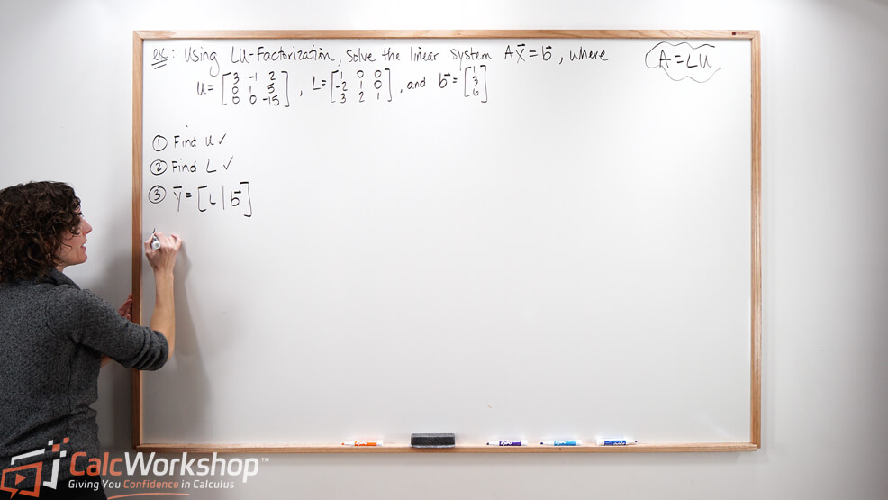
We’ll use LU factorization to solve the linear system in the following format:

\begin{aligned}
A \vec{x} &= \vec{b} \\
A &= \left[\begin{array}{ccc}3 & -1 & 2 \\ -6 & 3 & 1 \\ 9 & -1 & 1\end{array}\right] \\
\vec{b} &= \left[\begin{array}{l}1 \\ 3 \\ 6\end{array}\right]
\end{aligned}

First, we will find our upper triangular matrix (U) and lower triangular matrix (L) using the steps seen above.

\begin{aligned}
U &= \left[\begin{array}{ccc}3 & -1 & 2 \\ 0 & 1 & 5 \\ 0 & 0 & -15\end{array}\right] \\
\text{and} \\
L &= \left[\begin{array}{ccc}1 & 0 & 0 \\ -2 & 1 & 0 \\ 3 & 2 & 1\end{array}\right]
\end{aligned}

Next, we solve the system \(L y=\vec{b}\)

\begin{equation}
\left[\begin{array}{ccc}
1 & 0 & 0 \\
-2 & 1 & 0 \\
3 & 2 & 1
\end{array}\right]\left[\begin{array}{l}
y_1 \\
y_2 \\
y_3
\end{array}\right]=\left[\begin{array}{l}
1 \\
3 \\
6
\end{array}\right] \Rightarrow \begin{aligned}
& y_1=1 \\
& -2 y_1+y_2=3 \\
& 3 y_1+2 y_2+y_3=6
\end{aligned}
\end{equation}

By using forward substitution, we can solve for the missing y-variables

\begin{equation}
\begin{gathered}
y_1=1 \\
-2 y_1+y_2=3 \quad \rightarrow \quad-2(1)+y_2=3 \quad \rightarrow \quad y_2=5 \\
3 y_1+2 y_2+y_3=6 \rightarrow 3(1)+2(5)+y_3=6 \quad \rightarrow \quad y_3=-7
\end{gathered}
\end{equation}

Thus, \(y=\left[\begin{array}{c}1 \\ 5 \\ -7\end{array}\right]\)

Now, it’s time to find the original system, so we solve \(\vec{u}=y\)

\begin{equation}
\left[\begin{array}{ccc}
3 & -1 & 2 \\
0 & 1 & 5 \\
0 & 0 & -15
\end{array}\right]\left[\begin{array}{l}
x_1 \\
x_2 \\
x_3
\end{array}\right]=\left[\begin{array}{c}
1 \\
5 \\
-7
\end{array}\right] \Rightarrow \begin{aligned}
& 3 x_1-x_2+2 x_3=1 \\
& x_2+5 x_3=5 \\
& -15 x_3=-7
\end{aligned}
\end{equation}

This time we will use backward substitution to solve of \(\mathrm{x}\).

\begin{equation}
\begin{aligned}
3 x_1-x_2+2 x_3 & = 1 \\
& \rightarrow 3 x_1-\left(\frac{8}{3}\right)+2\left(\frac{7}{15}\right)=1 \\
& \rightarrow x_1=\frac{41}{45}
\end{aligned}
\end{equation}

\begin{equation}
\begin{aligned}
x_2+5 x_3 & = 5 \\
& \rightarrow x_2+5\left(\frac{7}{15}\right)=5 \\
& \rightarrow x_2=\frac{8}{3}
\end{aligned}
\end{equation}

\begin{equation}
\begin{aligned}
-15 x_3 & =-7 \\
& \rightarrow x_3=\frac{7}{15}
\end{aligned}
\end{equation}

\begin{equation}
\text { Hence, } \vec{x}=\left[\begin{array}{c}
41 / 45 \\
8 / 3 \\
7 / 15
\end{array}\right]
\end{equation}

Next Steps

In this video lesson, you will:

• Learn the two methods for LU factorization
• Use matrix decomposition to solve matrix equations \(\mathrm{Ax}=\mathrm{b}\)

Get ready for a fun learning experience!

Video Tutorial w/ Full Lesson & Detailed Examples

Get access to all the courses and over 450 HD videos with your subscription

Monthly and Yearly Plans Available

Get My Subscription Now

Still wondering if CalcWorkshop is right for you?
Take a Tour and find out how a membership can take the struggle out of learning math.