Log Transformation
The Why, When, & How (w/ Examples!)

What is a log transformation?

Great question!

It’s one of several methods that you can use to transform datasets to achieve linearity .

This means it can help you obtain further insights into your data that may not be obvious at first.

Let’s jump in!

Okay, so we know that a lack of linearity implies a lack of association, but is there a way to transform one or both of the variables so that a nonlinear relationship can be changed into a linear relationship?

When observation, theory, or experience suggests that the explanatory and response variables follow a familiar model.

What are the common types of transformations to achieve linearity?

• Power Model
• Exponential Model
• Square Root Model
• Logarithmic Model
• Hyperbolic Model

How do we transform the nonlinear quantitative variables to create a linear relationship? In other words, how do we linearize a curved pattern?

We apply one of the desired transformation models to one or both of the variables. For example, if we choose the logarithmic model, we would take the explanatory variable’s logarithm while keeping the response variable the same. In contrast, the power model would suggest that we log both the x and y variables.

Determining the right model to choose is easiest to determine after looking at a scatterplot of the data. Then, depending on the curved pattern displayed, and whether or not the origin, is a data point, it will allow you to select the best transformation model to achieve linearity.

And once we have transformed the sample data to achieve linearity, we can then find the least-squares regression line and verify our results with a residual plot.

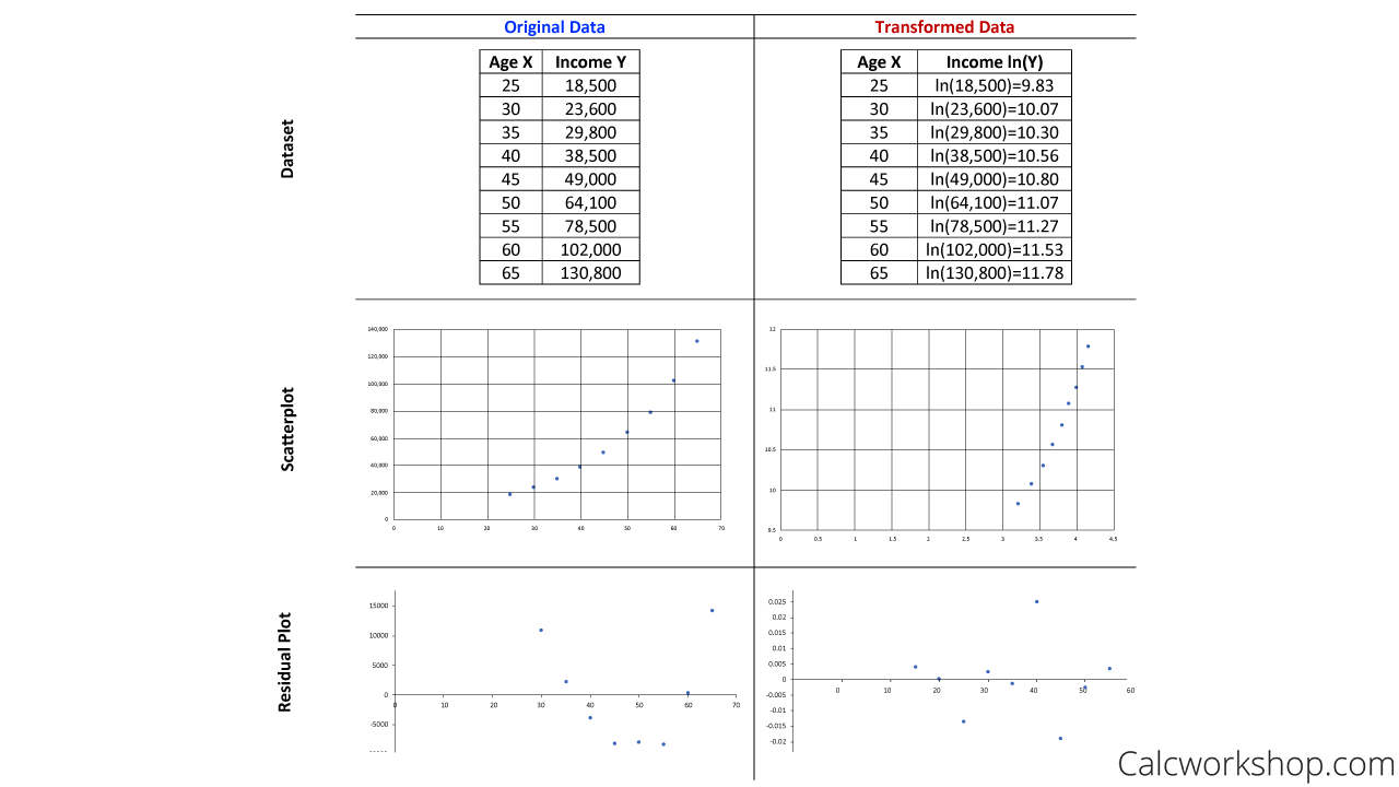
For example, notice how the original data below shows a nonlinear relationship. Well, after applying an exponential transformation, which takes the natural log of the response variable, our data becomes a linear function as seen in the side-by-side comparison of both scatterplots and residual plots.

It is always important to note that the results we obtain are only as good as the transformation model we assume as discussed by UVA.

Therefore, it’s still important to compare the coefficient of determination for the transformed values with the original values and choose a transformation with a high R-squared value.

Together we will look at how to transform data sets using all of the most common linear transformations. And we will learn how to write a least-squares regression equation for the transformed data, as well as how to graph residual plots and determine the coefficient of determination using technology.

Log Transformation – Lesson & Examples (Video)

31 min

• Introduction to Video: Transformation to Achieve Linearity
• 00:00:26 – Why and How do we transform data to achieve linearity?
• Exclusive Content for Members Only

• 00:08:14 – Given a data set find the regression line, r-squared value, and residual plot (Example #1)
• 00:12:57 – Use the Power transformation to find the transformed regression line, r-squared value and residual plot (Example #1a)
• 00:16:30 – Use the Exponential transformation to find the transformed regression line, r-squared value and residual plot (Example #1b)
• 00:19:30 – Use the Square Root transformation to find the transformed regression line, r-squared value and residual plot (Example #1c)
• 00:21:51 – Use the Log and Hyperbolic transformations to find the transformed regression line, r-squared value and residual plot (Example #1d and 1e)
• 00:24:44 – Use regression analysis to determine the best answer (Example 2)
• 00:26:46 – Transform using the square root or logarithmic method and use the transformed data to predict a future value (Example #3)
• Practice Problems with Step-by-Step Solutions
• Chapter Tests with Video Solutions