Least Squares Regression Line
w/ 19 Worked Examples!

Did you know that the least squares regression line can be used to predict future values?

Jenn, Founder Calcworkshop^®, 15+ Years Experience (Licensed & Certified Teacher)

Now that’s pretty amazing!

In fact, a least squares regression line (LSRL) helps us to measure the trend and relationship of collected data values and allows us to answer questions like…

• What happens when we want to study two variables at one time?
• What is their relationship?
• Is there an association that exists?
• What is the strength of the association, if any, and how can it be measured?
• Is there a way to measure and express this relationship mathematically, and then use this equation to predict future values?

All of these questions, and more, can be expressed using regression as it is a “best fit” for the data!

And that’s why least squares regression is sometimes called the line of best fit.

Now, regression analysis on bivariate (two-variable) data, has several key aspects that all help us to explain association and predict relationships:

1. Scatterplots
2. Correlation
3. Least-Squares Regression Lines
4. Residuals
5. Residual Plots

Scatterplots

Scatterplots are a way for us to visually display a relationship between two quantitative variables, typically written in the form (x,y), where x is the explanatory or independent variable, and y is the response or dependent variable.

Additionally, scatterplots help us to identify outliers and influential points.

Correlation

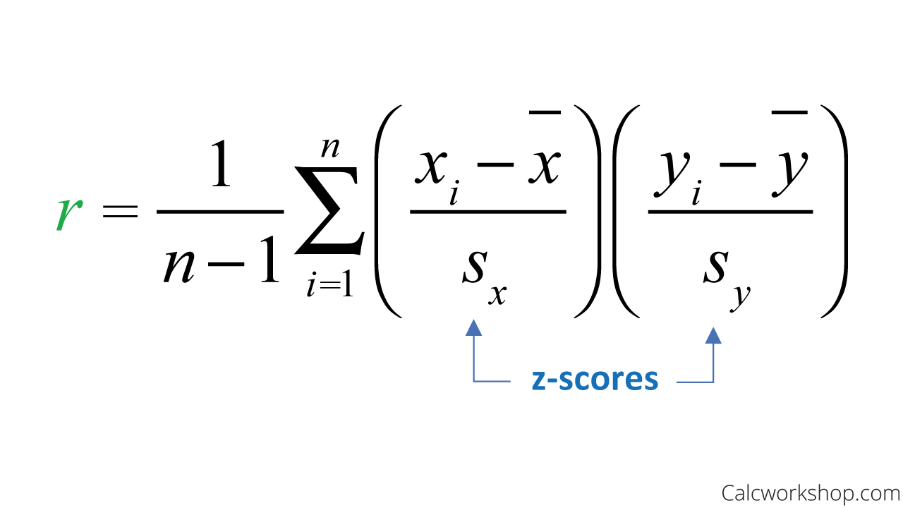
Correlation Coefficient Formula

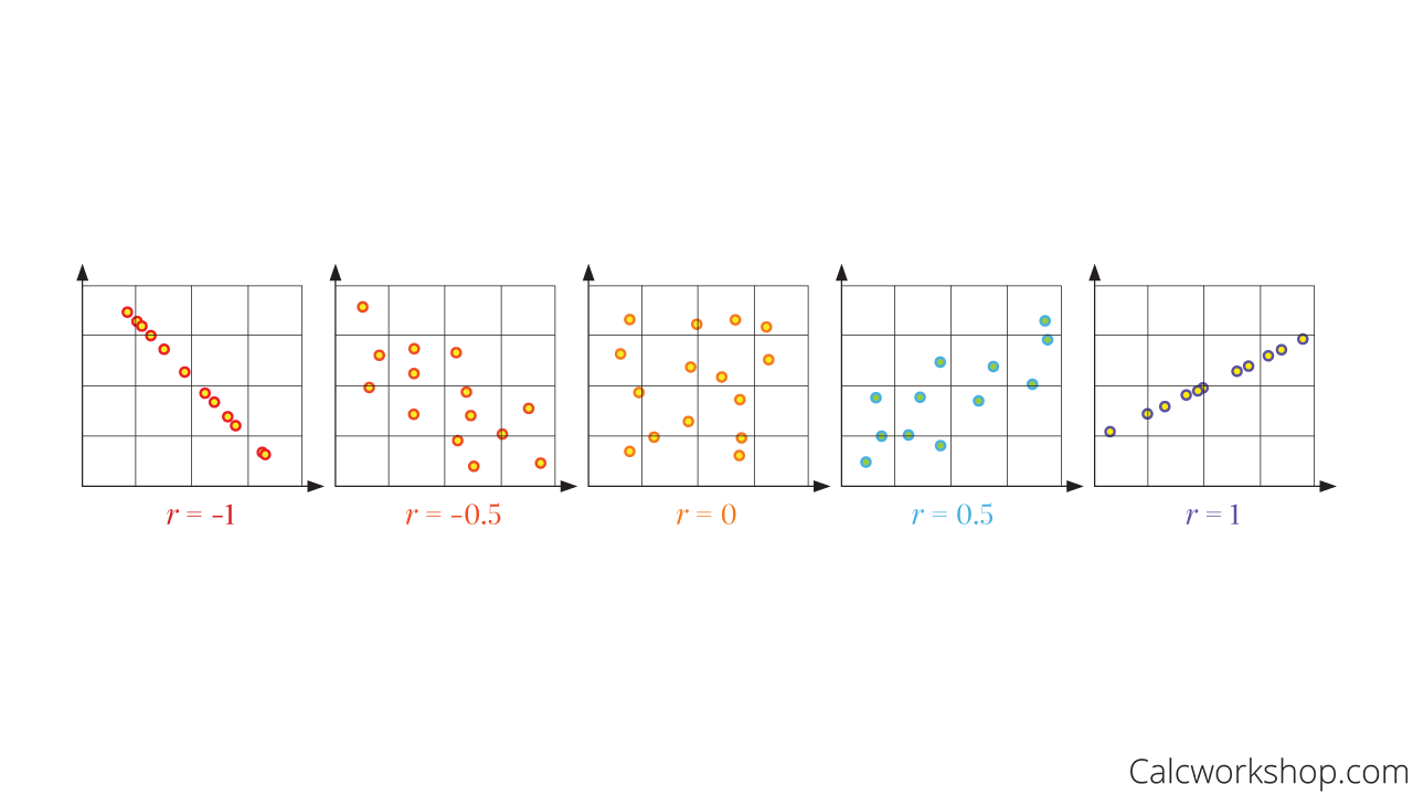
Correlation Coefficient Interpretation

Least-Squares Regression Lines

And if a straight line relationship is observed, we can describe this association with a regression line, also called a least-squares regression line or best-fit line. This trend line, or line of best-fit, minimizes the predication of error, called residuals as discussed by Shafer and Zhang. And the regression equation provides a rule for predicting or estimating the response variable’s values when the two variables are linearly related.

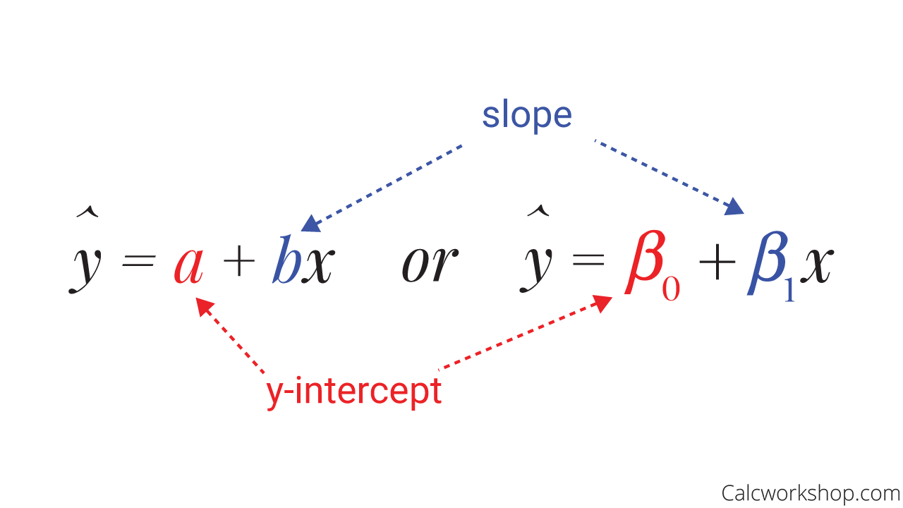
Least Squares Regression Line Equation

We will observe that there are two different methods for calculating the LSRL, depending on whether we are given raw data or summary statistics. But what is important to note about the formulas shown below, is that we will always find our slope (b) first, and then we will find the y-intercept (a) second.

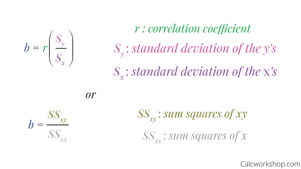
Slope Formulas for LSRL (Summary Statistics vs Raw Data)

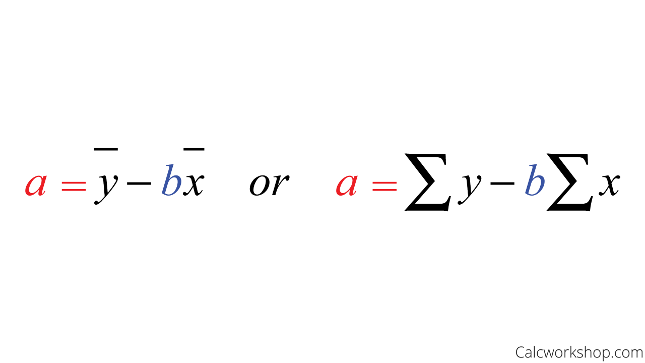
Y Intercept Formulas For LSRL (Raw Data vs Summary Statistics)

Residuals

Now the residuals are the differences between the observed and predicted values. It measures the distance from the regression line (predicted value) and the actual observed value. In other words, it helps us to measure error, or how well our regression line “fits” our data. Moreover, we can then visually display our findings and look for variations on a residual plot.

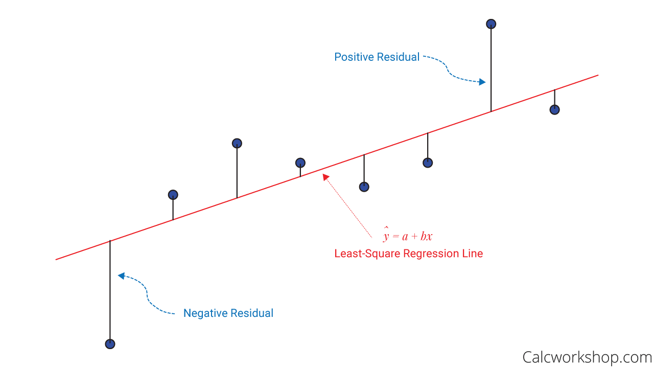
Residual Plot Interpretation

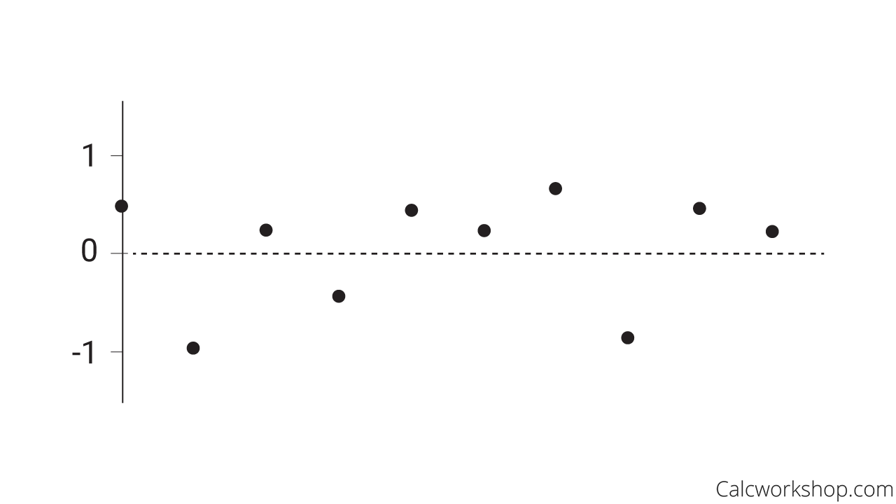
Residual Scatter Plot

Likewise, we can also calculate the coefficient of determination, also referred to as the R-Squared value, which measures the percent of variation that can be explained by the regression line.

But there is always a word of caution: correlation doesn’t necessarily imply causation. Just because there is a strong relationship, we must be careful not to conclude a cause and effect relationship between two variables or use our noticed association to extrapolate beyond the data.

Throughout our study, we will see that the least-squares regression equation is the line that best fits the sample data where the sum of the square of the residuals is minimized and fits the mean of the y-coordinates for each x-coordinate. Generally speaking, this line is the best estimate of the line of averages.

Worked Example

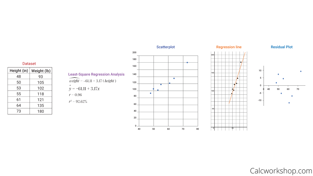
Together we use raw data as well as summary statistics to create scatterplots, regression analysis, find the LSRL, correlation coefficients, and determine if the analysis is a “good fit” by calculating the coefficient of determination, as the example below illustrates.

First we will create a scatterplot to determine if there is a linear relationship. Next, we will use our formulas as seen above to calculate the slope and y-intercept from the raw data; thus creating our least squares regression line. Then we will calculate our correlation coefficient to measure the strength of the relationship between the bivariate data and lastly we will determine the residuals, or error, from our predicted value to our observed value and construct a residual plot.

Finding LSRL for Dataset

Analyzing bivariate data has never been more fun!

Least Squares Regression Line – Lesson & Examples (Video)

2 hr 22 min

• Introduction to Video: Least-Squares Regression
• 00:00:38 – Identify Explanatory and Response Variables and How to determine the Correlation Coefficient (Example #1)
• Exclusive Content for Members Only

• 00:15:28 – Find the correlation coefficient using both formula methods (Example #2)
• 00:26:33 – Find the correlation coefficient and create a scatterplot (Example #3)
• 00:32:23 – Would you expect a positive, negative or no association for the pairs of variables (Example #4)
• 00:38:13 – Consider the scatterplot and determine the linear association (Example #5)
• 00:39:59 – How to find the Least Squares Regression Line using raw data or summary statistics
• 00:50:28 – Find the LSRL (Examples #6-7)
• 01:01:13 – What are residuals, outliers and influential points? With Example #8
• 01:14:51 – Use the data to create a scatterplot and find the correlation coefficient, LSRL, residuals and residual plot (Example #9)
• 01:30:16 – Find the regression line and use it to predict a value (Examples #10-11)
• 01:36:59 – Using technology find the regression line, correlation coefficient, coefficient of determination and use the LSRL to predict a future value (Example #12-13)
• 01:53:21 – Using the regression line interpret the slope and r-squared value and find the residual (Example #14)
• 01:58:13 – Using output data determine the regression line (Example #15)
• 02:00:38 – Determine if the observation in a regression outlier and has influence on the regression analysis (Example #16)
• 02:06:06 – Explain what is wrong with the way regression is used in each scenario (Example #17)
• 02:12:40 – Construct a scatterplot and compute the regression line and determine correlation and coefficient of determination (Example #18)
• 02:18:29 – Find the regression line and use it to predict future values (Example #19)
• Practice Problems with Step-by-Step Solutions
• Chapter Tests with Video Solutions