Did you know that linear algebra is the study of linear equations using matrix arithmetic?

Jenn, Founder Calcworkshop®, 15+ Years Experience (Licensed & Certified Teacher)
But to explore matrices and their implications, we must first understand linear equations. In particular, systems of linear equations. The good thing is that you already know so much about studying linear equations from your previous work in Algebra and Precalculus.
Before we can springboard off to even greater depths of study, let’s:
- Make sure we remember the essential details related to linear systems
- Discuss some important, and possibly new, definitions and ideas
What does it mean for an equation to be linear?
Understanding Linear Equations
A linear equation is one where all the variables are to the first power. It is important to note that some textbooks refer to an exponent as an index.
Alright, let’s see if we can determine which of the following equations are linear.
Yes, this is a linear equation as all variables
Now, this is not a linear equation as the power of the
While it may at first appear that this equation is not linear due to the exponents on the variables, we can quickly see that this equation is indeed linear upon closer inspection and simplification. Recall, the Pythagorean identity
Okay, so now that we know what linear means, what is a linear system?
Exploring Linear Systems of Equations
A system of linear equations is about finding what two or more equations have in common. In other words, we are trying to find the point of intersection!
From our previous Algebra studies, we know that there are several ways for us to solve a system of equations:
- Graphing
- Substitution
- Elimination method (linear combination method)
And the values that satisfy a linear system are called the solution or the solution set.
A linear system of equations has either:
- No solution
- Exactly one solution
- Infinitely many solutions
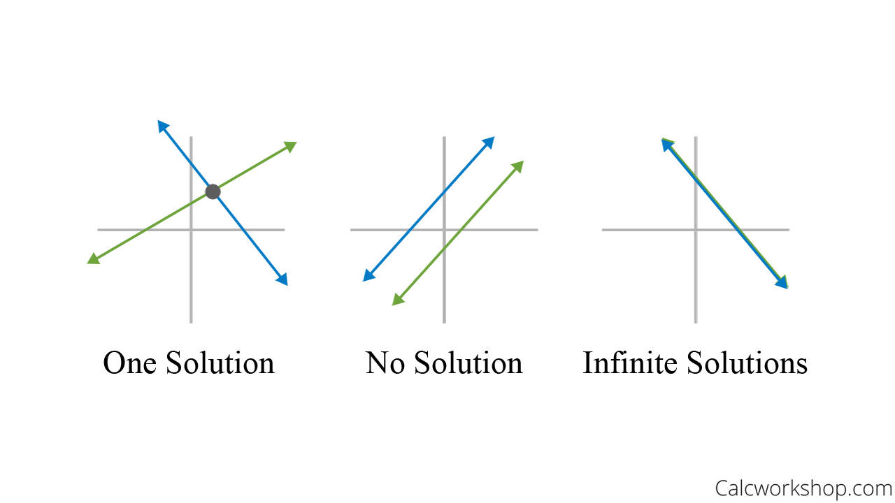
This is best indicated graphically, as shown in the figure below. Remember, if two lines intersect, the point of intersection gives the solution to the system and shows consistency. In contrast, two parallel lines yield an inconsistent system with no solution. And if the lines coincide (i.e., same line), there are infinite solutions.

Solutions for a System of Equations
Consistent and Inconsistent Systems
But what does it mean for a system to be consistent or inconsistent?
If a linear system has at least one solution, then it is considered consistent. And a system is said to be inconsistent if it has no solution. Therefore, using our graphs above, both one solution and infinitely many solutions are consistent.
It makes sense, right? But maybe you’re a little rusty with your system-solving methods. Never fear. Let’s practice a bit because knowing how to solve a system of equations is what Linear Algebra is all about.
In fact, solving a system of equations using the elimination method is one of the most essential skills you will need for this course. So, let’s dust off this valuable tool before adding more tools to our toolbelt.
Elimination Method for Solving Linear Systems
Solve the following system using the elimination process, or what is also commonly referred to as the process of linear combinations.
First, we align each equation, so that like variables are organized into columns.
Now it’s time to eliminate a variable. How?
If the coefficients of one variable are opposites, you add the equations to eliminate a variable and then solve.
But because neither of our variables are opposites, we must create opposites by multiplying one or both equations by a number to create opposite coefficients.
Next, we add the two equations together to eliminate a variable and solve.
Lastly, we substitute this value back into one of the original equations and solve for the other variable.
So, the solution to our system is
Now you may be thinking, what’s the point of “linear algebra” if I already know how to solve a system of linear equations?
Great question!
While linear algebra deals heavily with linear equations, it also encompasses:
- Vectors
- Transformations
- Networks
- and more
Additionally, our knowledge of solving linear equations is not quite robust enough to handle some more complex problems.
In other words, the graphing method, substitution method, or elimination method is sufficient for solving linear systems of two or possibly three equations with one, two, or three variables; it woefully lacks when we increase in the number of variables or equations.
What would you do if I asked you to solve a system with 500 variables or 500 equations?
Scream? Cry? Perhaps. Or maybe you just need a new tool in our toolbelt.
Introduction to Matrices
What new tool? Matrices!
Because a linear system can contain
Where
But here’s the key to solving systems – organization and focusing upon essential information.
A matrix is a rectangular array that contains only the essential information,
Augmented Matrices and Matrix Notation
The matrix above is called an augmented matrix, as it represents the coefficients of the unknown variables and the constant values on the right-hand side of the equations.
The size of a matrix tells us how many rows and columns it has. We let m represent the number of rows and
It’s important to note that the number of rows always comes first!
Additionally, some textbooks will use parentheses rather than brackets to represent a matrix.
Both brackets and parentheses are acceptable and interchangeable, as they are simply a personal preference.
Remember that while this notation may feel cumbersome initially, matrix notation will simplify our calculations significantly. Before you know it, the new matrices tool will feel comfortable and useful.
Next Steps
In fact, during this lesson, you will:
- Review linear systems and solving techniques
- Be introduced to matrices
- Explore the concepts of consistency vs. inconsistency
- Understand equivalence and uniqueness
This is just the beginning of a great adventure into Linear (Matrix) Algebra. Join in the video for the start of your epic journey.
Video Tutorial w/ Full Lesson & Detailed Examples

Get access to all the courses and over 450 HD videos with your subscription
Monthly and Yearly Plans Available
Still wondering if CalcWorkshop is right for you?
Take a Tour and find out how a membership can take the struggle out of learning math.