Sometimes, when we believe that someone or something is unimportant, we say they are trivial and do not need any serious concern.
But in mathematics, the opposite is true. In fact, the term “trivial” has huge importance, especially concerning the solution sets of linear systems.
Okay, so a system of linear equations is a collection of two or more equations where the number of equations is not required to be the same as the number of unknown variables. For example, a system of linear equations may look something like the following:
\begin{align*}
\begin{aligned}
& x_{1}-7 x_{2}+2 x_{3}-5 x_{4}+8 x_{5}=10 \\
& x_{2}-3 x_{3}+3 x_{4}+x_{5}=-5 \\
& x_{4}-x_{5}=4
\end{aligned}
\end{align*}
Now, the solution to the system above is the set of values for \(x_{1}, x_{2}, x_{3}, x_{4}\) and \(x_{5}\) that make the equations true. For instance, \(\left(x_{1}, x_{2}, x_{3}, x_{4}, x_{5}\right)=(-82,-15,2,5,1)\) is a solution to this system and can be verified by substituting these values into each question and obtaining a true statement.
And as our previous lesson showed us, we can write this system as a vector equation as follows.
\begin{align*}
x_{1}\left[\begin{array}{l}
1 \\
0 \\
0
\end{array}\right]+x_{2}\left[\begin{array}{c}
-7 \\
1 \\
0
\end{array}\right]+x_{3}\left[\begin{array}{c}
2 \\
-3 \\
0
\end{array}\right]+x_{4}\left[\begin{array}{c}
-5 \\
3 \\
1
\end{array}\right]+x_{5}\left[\begin{array}{c}
8 \\
1 \\
-1
\end{array}\right]=\left[\begin{array}{c}
10 \\
-5 \\
4
\end{array}\right]
\end{align*}
Homogeneous and Nonhomogeneous Systems
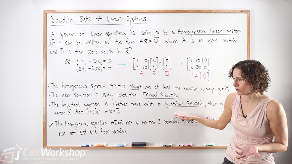
But did you know that a system of linear equations is considered homogenous if the “bs” or the right-hand side is the zero vector?
Imagine if our given system was written as follows.
\begin{align*}
\begin{aligned}
& x_{1}-7 x_{2}+2 x_{3}-5 x_{4}+8 x_{5}=0 \\
& x_{2}-3 x_{3}+3 x_{4}+x_{5}=0 \\
& x_{4}-x_{5}=0
\end{aligned}
\end{align*}
This means that our matrix equation would look something like this.
\begin{align*}
\left[\begin{array}{ccccc}
1 & -7 & 2 & -5 & 8 \\
0 & 1 & -3 & 3 & 1 \\
0 & 0 & 0 & 1 & -1
\end{array}\right]\left[\begin{array}{l}
x_{1} \\
x_{2} \\
x_{3} \\
x_{4} \\
x_{5}
\end{array}\right]=\left[\begin{array}{l}
0 \\
0 \\
0
\end{array}\right]
\end{align*}
Which is the same thing as saying \(A \vec{x}=\overrightarrow{0}\)
Now why is this important to know?
Importance of Trivial Solutions
Because while this homogeneous system has several solutions, it has one very special solution, namely \(\left(x_{1}, x_{2}, x_{3}, x_{4}, x_{5}\right)=(0,0,0,0,0)\)
\begin{align*}
\begin{aligned}
& x_{1}-7 x_{2}+2 x_{3}-5 x_{4}+8 x_{5}=0 \\
& x_{2}-3 x_{3}+3 x_{4}+x_{5}=0 \\
& x_{4}-x_{5}=0
\end{aligned} \rightarrow\left[\begin{array}{l}
x_{1} \\
x_{2} \\
x_{3} \\
x_{4} \\
x_{5}
\end{array}\right]=\left[\begin{array}{l}
0 \\
0 \\
0 \\
0 \\
0
\end{array}\right]
\end{align*}
This solution, which is a vector where all of its coordinates are 0, is called the trivial solution!
But, in Linear Algebra, we are never satisfied with finding just one solution to a system. We want to find all possible solutions. This is called the solution set.
Linear Independence and Solution Sets
Additionally, as we will see in future lessons, trivial and non-trivial solutions will play a critical role in determining linear independence.
Okay, so let’s ensure we’ve got a handle on our vocabulary before going any further.
A homogeneous system, \(\overrightarrow{A x}=\overrightarrow{0}\), of linear equations is when the system has only one solution (i.e., the trivial solution, which is the zero vector) or the system has more than one solution.
A nonhomogeneous system, \(\overrightarrow{A x}=\vec{b}\), of linear equations is when the system has a unique (single) solution, the system has more than one solution, or the system has no solution at all.
The trivial solution is the zero-vector solution, whereas a non-trivial solution is any solution other than the trivial one. As you will find as we progress through this course, knowing whether a solution has only the trivial solution is going to be of utmost importance as it pertains to linear independence, so being able to decipher between trivial and non-trivial solutions is critical.
Alright, so it is also important to note that a homogenous equation \(\overrightarrow{A x}=\overrightarrow{0}\) has a non-trivial solution if and only if the equation has at least one free variable.
This means, using our example above and performing reduced row echelon techniques, we are left with a non-trivial solution because we have three pivots and two free variables.
\begin{align*}
\left[\begin{array}{cccccc}
1 & -7 & 2 & -5 & 8 & 0 \\
0 & 1 & -3 & 3 & 1 & 0 \\
0 & 0 & 0 & 1 & -1 & 0
\end{array}\right] \sim\left[\begin{array}{cccccc}
1 & 0 & -19 & 0 & 31 & 1 \\
0 & 1 & -3 & 0 & 4 & 0 \\
0 & 0 & 0 & 1 & -1 & 0
\end{array}\right]
\end{align*}
But sometimes, this is hard for us to see.
So, wouldn’t it be great if we could write our solution set in a way that makes it obvious which variables are the free variables?
Parametric Vector Form for Solution Sets
Good thing we have something called Parametric Vector Form!
With parametric vector form, we will take an implicit description of the solution and find an explicit description using parametric vector form.
How?
Let’s use our original matrix from above where \(\overrightarrow{A x}=\vec{b}\) to demonstrate the process.
\begin{aligned}
x_{1} & -7 x_{2}+2 x_{3}-5 x_{4}+8 x_{5}=10 \\
x_{2} & -3 x_{3}+3 x_{4}+x_{5}=-5 \\
x_{4} & -x_{5}=4
\end{aligned}
First, we will row reduce the augmented matrix to reduce row echelon form.
\begin{align*}
\left[\begin{array}{cccccc}
1 & -7 & 2 & -5 & 8 & 10 \\
0 & 1 & -3 & 3 & 1 & -5 \\
0 & 0 & 0 & 1 & -1 & 4
\end{array}\right] \sim\left[\begin{array}{cccccc}
1 & 0 & -19 & 0 & 31 & -89 \\
0 & 1 & -3 & 0 & 4 & -17 \\
0 & 0 & 0 & 1 & -1 & 4
\end{array}\right]
\end{align*}
Next, we will transform the general solution by expressing each basic variable (pivot) in terms of any free variables.
\begin{equation}
\begin{array}{lc}
x_1-19 x_3+31 x_5=-89 \\
x_2-3 x_3+4 x_5=-17 \\
x_4-x_5=4
\end{array} \rightarrow \quad \begin{gathered}
x_1=-89+19 x_3-31 x_5 \\
x_2=-17+3 x_3-4 x_5 \\
x_4=4+x_5
\end{gathered}
\end{equation}
Right off the bat, we can now see that the basic variables are \(x_{1}, x_{2}, x_{4}\) and the free variables are \(x_{3}\) and \(x_{5}\).
\begin{aligned}
x_1 & =-89+19 x_3-31 x_5 \\
x_2 & =-17+3 x_3-4 x_5 \\
x_4 & =4+x_5
\end{aligned}
\begin{equation}
\longrightarrow
\end{equation}
\begin{aligned}
x_1 & =19 x_3-31 x_5 \\
x_2 & =-17+3 x_3-4 x_5 \\
x_3 & =x_3 \\
x_4 & =4+x_5 \\
x_5 & =x_5
\end{aligned}
So, now it’s time to take our implicit solution and write it explicitly by decomposing \(\vec{x}\) into a linear combination of vectors using the free variables as parameters!
\begin{align*}
\vec{x}=\left[\begin{array}{c}
-89 \\
-17 \\
0 \\
4 \\
0
\end{array}\right]+x_{3}\left[\begin{array}{c}
19 \\
3 \\
1 \\
0 \\
0
\end{array}\right]+x_{5}\left[\begin{array}{c}
-31 \\
-4 \\
0 \\
1 \\
1
\end{array}\right]
\end{align*}
Notice that this looks very similar to how we write equations of lines for vectors.
\begin{align*}
\vec{x}=\langle\text { point }\rangle+t\langle\text { vector }\rangle=\vec{p}+\overrightarrow{v_{h}}
\end{align*}
What this means is that the solution set of \(\overrightarrow{A x}=\vec{b}\) is the set of all vectors of the form \(\vec{x}=\vec{p}+\overrightarrow{v_{h}}\), where \(\overrightarrow{v_{h}}\) is any solution of the homogenous equation \(\overrightarrow{A x}=\overrightarrow{0}\), and the vector equation above represents the line through point, \(\vec{p}\) parallel to the set of all vectors \(\overrightarrow{v_{h}}\).
Cool!
Together we will learn some fundamental definitions and vocabulary for the study of Matrix Algebra, determine whether a system has a trivial or non-trivial solution, and describe solutions in parametric vector form.
It’s going to be great, so let’s get to it!
Video Tutorial w/ Full Lesson & Detailed Examples
Get access to all the courses and over 450 HD videos with your subscription
Monthly and Yearly Plans Available
Still wondering if CalcWorkshop is right for you?
Take a Tour and find out how a membership can take the struggle out of learning math.