Reduced Row Echelon Form
A Key Tool for Matrix Operations

What if I told you you already know the steps for finding the reduced row echelon form?

It’s true!

Everything you need to know comes from our knowledge of solving systems of equations using the elimination method!

Recall that the elimination method for solving linear systems has three components:

1. Multiply an equation by a non-zero constant (i.e., scalar)
2. Add a multiple of one equation to another.
3. Interchange equations

Elementary Row Operations

So, guess what?

These are the exact three operations we will use when performing elementary row operations for a matrix!

What’s an elementary row operation?

Row operations are an algorithm or a set of procedures. They are the calculations we use to solve a system of equations in matrix form. The only difference is that instead of saying “equation,” we use the word “row” because each row represents those essential elements from each equation.

And as stated earlier, there are only three row reducing techniques:

1. Multiply a row by a non-zero constant (i.e., scalar)
2. Add a multiple of one row to another.
3. Interchange rows

Okay, but what’s the point of row reduction?

Well, just like we say with the elimination method from Algebra, our ultimate goal is to solve the system of equations. We do this by transforming our equations (i.e., rows) into a more simplified equivalent matrix.

Example: Elimination Method vs. Row Operations

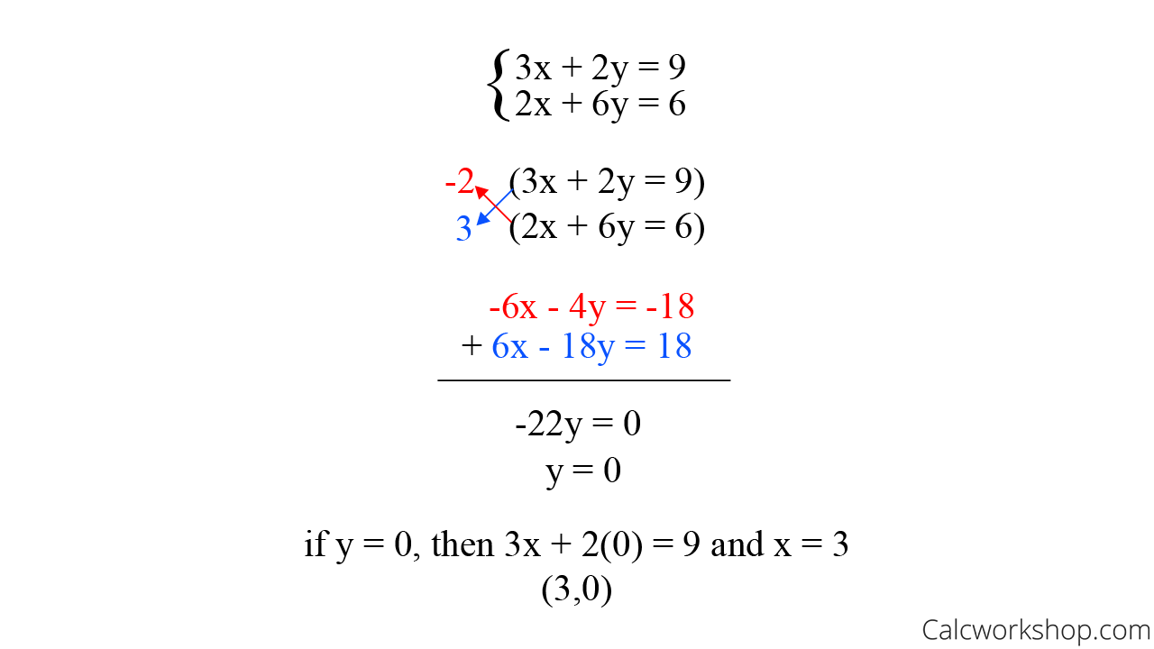
For example, let’s take the following system and solve using the elimination method steps.

But now, let’s do the same thing, but this time we’ll use matrices and row operations.

First, we will transform the system of equations into an augmented matrix, as we learned in our previous lesson.

Remember, an augmented matrix is a shorthand way of representing a system of linear equations that only focuses on the essential elements (i.e., coefficients and constants) while ignoring the variables in order to make arithmetic and analysis easier.

\begin{align*}
\begin{aligned}
& 3 x+2 y=9 \\
& 2 x+6 y=6
\end{aligned} \Rightarrow\left[\begin{array}{lll}
3 & 2 & 9 \\
2 & 6 & 6
\end{array}\right]
\end{align*}

Next, we will add a multiple of one row to another. In other words, let’s add the first and second rows and replace the second row with our sum.

\begin{align*}
\left[\begin{array}{ccc}
-6 & -4 & -18 \\
6 & -18 & 18
\end{array}\right] \sim\left[\begin{array}{ccc}
3 & 2 & 9 \\
0 & -22 & 0
\end{array}\right]
\end{align*}

Now we will multiply the second row by a non-zero constant (i.e., scalar)

\begin{align*}
\left[\begin{array}{ccc}
-6 & -4 & -18 \\
0 & -22\left(\frac{-1}{22}\right) & 0\left(\frac{-1}{22}\right)
\end{array}\right] \sim\left[\begin{array}{ccc}
3 & 2 & 9 \\
0 & 1 & 0
\end{array}\right]
\end{align*}

Finally, we can rewrite the general solution of our matrix as a system of equations and employ back substitution to find our solution.

\begin{equation}
\left[\begin{array}{lll}
3 & 2 & 9 \\
0 & 1 & 0
\end{array}\right] \Rightarrow \begin{gathered}
3 x+2 y=9 \\
y=0
\end{gathered} \Rightarrow \begin{gathered}
3 x+2(0)=9 \\
3 x=9 \\
x=3
\end{gathered}
\end{equation}

See how row operations are similar to the elimination process, except we ignore the variables and focus on the numbers?

If this still seems a bit fuzzy or confusing, don’t worry! In this video lesson, we teach you all the tricks for using Row Reduction and Echelon Forms to perfection.

But before we jump into the lesson, we need to talk about some important terminology we will use from this point forward.

Identity Matrices and Their Importance

Our study begins with an understanding of the Identity Matrix and how it is useful in determining a solution. Recall how the identity property in Algebra states that if you multiply any value by 1, it stays the same (i.e., \(a \cdot 1=a\) )?

Well, the identity matrix in Linear Algebra is a square matrix that behaves in the same manner. The main diagonal of the matrix is all \(1 \mathrm{~s}\), and every other element in the array are zeros. Here are some examples of identity matrices.

\begin{align*}
I=\left[\begin{array}{ll}
1 & 0 \\
0 & 1
\end{array}\right] \quad I=\left[\begin{array}{lll}
1 & 0 & 0 \\
0 & 1 & 0 \\
0 & 0 & 1
\end{array}\right] \quad I=\left[\begin{array}{cccc}
1 & 0 & \cdots & 0 \\
0 & 1 & \cdots & 0 \\
\vdots & \vdots & \ddots & \vdots \\
0 & 0 & \cdots & 1
\end{array}\right]
\end{align*}

Now, while we will learn about other beneficial aspects of the identity matrix in future lessons, one question begs to be asked. Why are identity matrices essential for solving systems?

Because this is what we are trying to achieve with row reduction – something that looks similar to the identity matrix! We want to take our given augmented matrix and transform it using our three-step algorithm to produce an equivalent matrix that looks like the identity matrix.

Echelon Form and Reduced Row Echelon Form

In doing so, we create what is called echelon form and reduced echelon form.

Echelon form, sometimes called Gaussian elimination or REF, is a transformation of the augmented matrix to a point where we can use backward substitution to find the remaining values for our solution, as we say in our example above.

The following matrices are in echelon form (REF). Notice how the leading entries (1) may have any non-zero value above, indicated by (*) and 0 s below.

\begin{align*}
\left[\begin{array}{ll}
1 & * \\
0 & 1
\end{array}\right],\left[\begin{array}{lll}
1 & * & * \\
0 & 1 & * \\
0 & 0 & 0
\end{array}\right],\left[\begin{array}{llll}
1 & * & * & * \\
0 & 1 & * & * \\
0 & 0 & 1 & * \\
0 & 0 & 0 & 0
\end{array}\right]
\end{align*}

Reduced echelon form, sometimes called Gauss-Jordan elimination or more commonly referred known as reduced row echelon form (RREF), is a steplike pattern that moves down and to the right through the matrix that looks strikingly similar to the identity matrix.

The matrices below are in reduced row echelon form (RREF). Notice how the leading entries (1), and there are 0 s above and below each leading 1.

\begin{align*}
\left[\begin{array}{lll}
1 & 0 & * \\
0 & 1 & *
\end{array}\right],\left[\begin{array}{llll}
1 & 0 & * & * \\
0 & 1 & * & * \\
0 & 0 & 0 & 0
\end{array}\right],\left[\begin{array}{llll}
1 & 0 & 0 & * \\
0 & 1 & 0 & * \\
0 & 0 & 1 & * \\
0 & 0 & 0 & 0
\end{array}\right]
\end{align*}

Both the Echelon form and Reduced Row Echelon form are useful to our study of matrices, but you will quickly find that while RREF may take a bit more work to achieve, it is the most preferred equivalent matrix form, as it yields the most desirable results.

Uniqueness Theorem and Pivot Positions

In fact, the uniqueness theorem for reduced echelon form states that each matrix is row equivalent to one and only one reduced row echelon form. While there may be more than one way to simplify or reduce a matrix, there will only be one final answer.

Why is this important?

Suppose you and your friend are tasked with solving a system of equations, but while you use one technique, your friend uses another. But regardless of how you went about solving the system, you both get the exact same final answer. That’s why it’s important! This gives you the freedom to “beat to your own drum,” knowing that you’ll get the correct answer, even if your method of solving differs from your neighbor! Gosh, math is cool!

Additionally, we will be referring to those “leading entries (1)” as Pivots and the column in which they reside are called pivot columns. These pivot columns correspond to the variables from the original system and are linearly independent.

Consequently, a pivot is an independent variable, sometimes called a basic variable, and a non-pivot is a dependent variable, which we call a free variable.

Don’t worry. I know this may seem overwhelming but trust me when I tell you that I’ve got many helpful hints and tricks (tips that aren’t found in textbooks) that will enable you to row reduce like a pro and make sense of the new terminology!

Next Steps

In this tutorial, you will:

• Learn the sequence of operations performed on the associated matrix of coefficients
• Define pivot positions and columns in detail
• Understand how to write a general solution
• Distinguish between basic variables and free variables
• Master the necessary skills of REF and RREF

Get ready for a fun learning journey. Let’s dive in!

Video Tutorial w/ Full Lesson & Detailed Examples

• How do we solve a system of linear equations?
• Understanding and Importance of the Identity Matrix
• Understanding Row Echelon Form and Reduced Row Echelon Form
• What is a Pivot Position and a Pivot Column?
• Steps and Rules for performing the Row Reduction Algorithm
• Example #1 Solving a system using Linear Combinations and RREF
• Example #2 Solving a system using REF
• Example #3 Solving a system using RREF

---

Get more examples and over 450 HD videos with your subscription

Monthly and Yearly Plans Available

Get My Subscription Now

Still wondering if CalcWorkshop is right for you?
Take a Tour and find out how a membership can take the struggle out of learning math.