Linear Transformations
Bridging - Theory and Practice

Have you ever tried to peer through a dirty window? Have your glasses, sunglasses, or possibly your car windshield been so fogged up that you can’t see through? Isn’t trying to understand what’s on the other side difficult in times like this?

As we learned in previous lessons, shifting our focus from a system of equations to vector or even matrix equations helps us better analyze the solution and provide a better view. We never actually changed the linear system; we just wrote it in such a way as to make it easier to see – we cleaned it up a bit or turned on the defrost.

However, there are other times when a simple defogging isn’t enough, and we need a bit more “umff!” and a little more action. We don’t just want to clean it up, but to truly transform it!

Matrix Equations and Transformations

The matrix equation \(A \vec{x}=\vec{b}\) gains power when we think of the matrix \(\mathrm{A}\) as an object that “acts” on a vector \(\vec{x}\) through multiplication; thus, causing a transformation or mapping.

Connections Between Geometry and Linear Algebra

Do you remember how in geometry, we learned that transformations occur when there is a change in size, shape, or position (i.e., dilation, rotation, reflection, and translation)? Now you may wonder, how does our knowledge of geometry and transformation relate to linear algebra?

Great question! Let’s dive into it.

• Transformation is a function or mapping that takes an input and produces an output. The fascinating part is that this transformation can be expressed by a matrix and interpreted similarly.
• Confused? Let’s break it down. Just like \(f(x)=\sqrt{x}\) is a function that accepts a value, x, as its input and spits out the square root of that number (i.e., \(f(9)=\sqrt{9}=3\), where the input is 9, and the output is 3), matrices behave the same as functions.

Matrix as Functions

Therefore, \(A \vec{x}=\vec{b}\), similar to \(y=f(x)\), can be thought of as a function where \(\mathrm{A}\) is the function with independent variable \(\vec{x}\) (i.e., input) and \(\vec{b}\) is the dependent variable (output). This means \(\mathrm{A}\) performs an action similar to how the square root acts on a number and transforms one real number into another.

Transformations in Linear Algebra

So, a transformation \(\mathrm{T}\) is a rule or action that assigns to each vector \(\vec{x}\) in \(\mathbb{R}^{n}\) a vector \(T(\vec{x})\) in \(\mathbb{R}^{m}\). Thus, we can define the following:
\begin{aligned}
\mathbb{R}^{n} & \text{ is the domain of } T \\
\mathbb{R}^{m} & \text{ is the codomain of } T \\
T(\vec{x}) & \text{ in } \mathbb{R}^{m} \text{ is the image of } \vec{x} \text{ under } T \\
\left\{T(\vec{x}): \vec{x} \text{ in } \mathbb{R}^{n}\right\} & \text{ in } \mathbb{R}^{m} \text{ is the range of } T \\
\end{aligned}

Codomain and Range

Wait! What’s the difference between codomain and range? Aren’t they the same thing?

Well, in your previous courses, the range and the codomain probably were the same, but the distinction is quite important as you progress in mathematics. The codomain is all the possible outcomes, while the range is all the actual outcomes (images) that appear after the transformation.

So, if \(T(\vec{x})=A \vec{x}\) where \(\mathrm{A}\) is an m x n matrix, then a matrix transformation, which is sometimes abbreviated by \(\vec{x} \mapsto A \vec{x}\), behaves something like this:

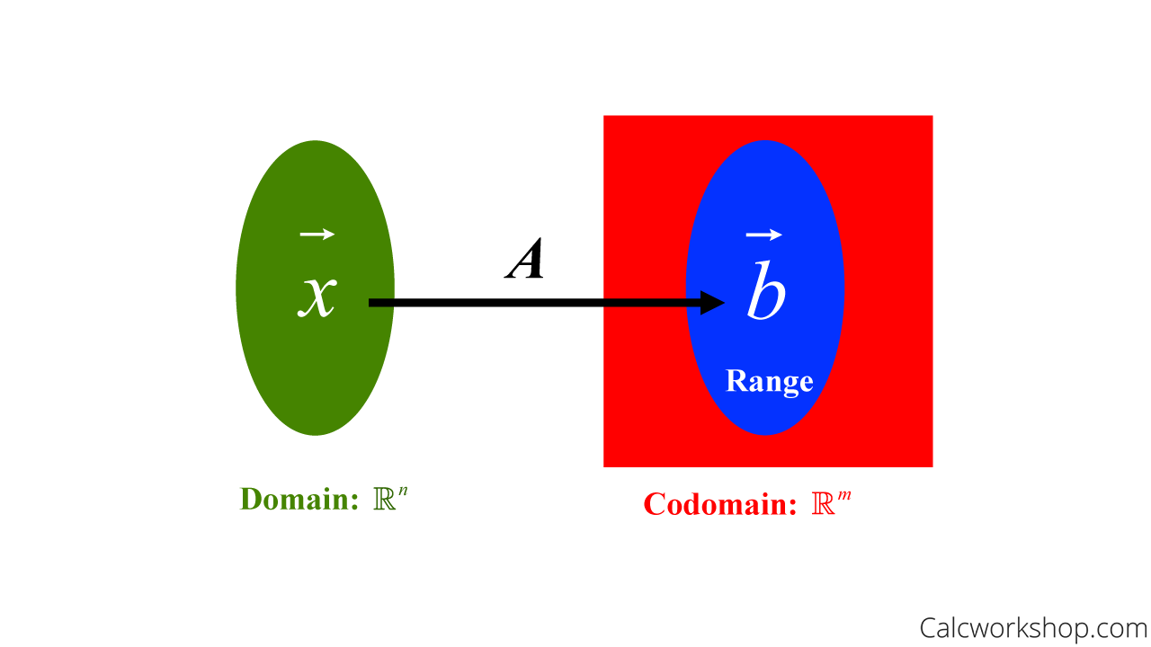
The green oval is the input value, the red square is all the possible outcomes, and the blue oval represents the range, all the actual outputs (images) that are calculated after the transformation A.

More specifically, if A is an mxn matrix, and \(T(\vec{x})=A \vec{x}\) is the matrix transformation, then:

• The domain of \(T\) is the number of columns (n) of A
• The codomain is the number of rows (m) of A
• The range is the column space of A

Don’t worry about understanding “column space” for now…we’ll come back to it in a future lesson, but for now, just know that the range of \(T\) is the set of all linear combinations \(\mathrm{s}\) of the columns of A.

Also, it may be helpful to point out that some textbooks refer to matrix A as the standard matrix for the linear transformation \(T\).

One-to-One and Onto Transformations

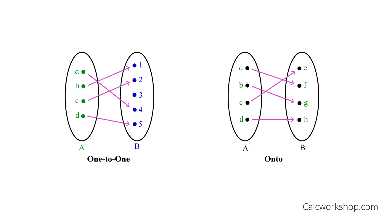
Now it’s time to talk about one-to-one (also known as injective) and onto (also known as surjective) transformations.

For a function to be one-to-one, every distinct element in the domain has a distinct image in the codomain. All this means is that every element in the domain (the green oval from the diagram above) maps to a “unique buddy” in the codomain.

Definition: A mapping \(T: \mathbb{R}^{n} \rightarrow \mathbb{R}^{m}\) is said to be one-to-one if each \(\vec{b}\) in \(\mathbb{R}^{m}\) is the image of at most one \(\vec{x}\) in \(\mathbb{R}^{n}\).

Now, an onto function is when every element in the codomain is mapped to by at least one element in the domain. Which means nothing in the codomain is left out. Simply put, an onto function is when the range equals the codomain (the blue oval is the same as the red square)!

Definition: A mapping \(T: \mathbb{R}^{n} \rightarrow \mathbb{R}^{m}\) is said to be onto if each \(\vec{b}\) in \(\mathbb{R}^{m}\) is the image of at least one \(\vec{x}\) in \(\mathbb{R}^{n}\).

Here’s a tip for keeping this straight … focus on the codomain and ask yourself how often each element gets mapped to, or as I like to say, how often each element gets “hit” or tagged.

• Injective (one-to-one): elements in the codomain get “hit” at most once
• Surjective (onto): elements in the codomain get “hit” at least once

Matrix Transformation Theorems

We have special theorems for one-to-one matrix transformations and onto matrix transformations that will help us perform and identify linear transformations.

One-to-One Matrix Transformation Theorem: If \(\mathrm{A}\) is an mxn matrix and let \(T(\vec{x})=A \vec{x}\) be a matrix transformation, then the following statements are equivalent:

• \(\mathrm{T}\) is one-to-one
• For every \(\vec{b}\) in \(\mathbb{R}^{m}\), the equation \(T(\vec{x})=\vec{b}\) has at most one solution
• For every \(\vec{b}\) in \(\mathbb{R}^{m}\), the equation \(A \vec{x}=\vec{b}\) has a unique solution or is inconsistent \(A \vec{x}=\overrightarrow{0}\) has only the trivial solution (zero vector)
• The columns of \(\mathrm{A}\) are linearly independent
• \(\mathrm{A}\) has a pivot in every column.
• The range of \(\mathrm{T}\) has dimension \(\mathrm{n}\).

Onto Matrix Transformation Theorem: If \(\mathrm{A}\) is an mxn matrix and let \(T(\vec{x})=A \vec{x}\) be a matrix transformation, then the following statements are equivalent:

• \(\mathrm{T}\) is onto
• \(T(\vec{x})=\vec{b}\) has at least one solution for every \(\vec{b}\) in \(\mathbb{R}^{m}\)
• \(A \vec{x}=\vec{b}\) is consistent for every \(\vec{b}\) in \(\mathbb{R}^{m}\)
• The columns of \(\mathrm{A}\) span \(\mathbb{R}^{m}\)
• \(\mathrm{A}\) has a pivot in every row.
• The range of \(\mathrm{T}\) has dimension \(m\).

Linear Transformations

Okay, now that we’ve gotten all our definitions and theorems, let’s learn how to verify, identify, and compute linear and matrix transformations.

Don’t worry. You already have a leg up because of your geometry transformations (reflections, rotations, translation, and dilations).

Examples of Matrix Transformations

So, a transformation \(T: \mathbb{R}^{n} \rightarrow \mathbb{R}^{m}\) is linear if:

• \(T(\vec{u}+\vec{v})=T(\vec{u})+T(\vec{v})\) for all \(\vec{u}, \vec{v}\) in the domain of \(T\)
• \(T(c \vec{u})=c T(\vec{u})\) for all \(\vec{u}\) and scalars \(\mathrm{c}\)

This means that every linear transformation preserves the operations of vector addition and scalar multiplication. And why is this important? Because every linear transformation is a matrix transformation.

Moreover, a linear transformation is our formula or “action” that allows us to dilate, reflect, rotate, shear, project, and rotate, just like we did with objects in geometry!

Dilation, Reflection, and Shear Examples

Okay, so let’s look at a few examples to help us understand matrix transformations.

Example of a Dilation: If \(T: \mathbb{R}^{2} \rightarrow \mathbb{R}^{2}\) where \(T(\vec{x})=0.25 x\). Find a standard matrix A for \(T\).

We obtain the columns of \(\mathrm{A}\) by evaluating \(\mathrm{T}\) on the standard coordinate vectors \(e_{1}, e_{2}\) which are the columns of the \(2 \times 2\) identity matrix.

\begin{equation}
\begin{aligned}
T\left(e_1\right)
& =0.25 e_1 \\
& =0.25\left[\begin{array}{l}
1 \\
0
\end{array}\right] \\
& =\left[\begin{array}{c}
0.25 \\
0
\end{array}\right] \\\\
T\left(e_2\right)
& =0.25 e_2 \\
& =0.25\left[\begin{array}{l}
0 \\
1
\end{array}\right] \\
& =\left[\begin{array}{cc}
0 \\
0.25
\end{array}\right] \\
A
& =\left[\begin{array}{cc}
T\left(e_1\right) & T\left(e_2\right)
\end{array}\right] \\
& =\left[\begin{array}{cc}
0.25 & 0 \\
0 & 0.25
\end{array}\right]
\end{aligned}
\end{equation}

Example of a Reflection

Find the standard matrix A for \(\mathrm{T}\) if (a) \(T: \mathbb{R}^{2} \rightarrow \mathbb{R}^{2}\) reflects through the vertical axis, and (b) \(T: \mathbb{R}^{2} \rightarrow \mathbb{R}^{2}\) reflects through the horizontal axis.

Just like we did for the previous example, we will be obtaining the columns of A by evaluating \(\mathrm{T}\) on the standard coordinate vectors \(e_{1}, e_{2}\) which are the columns of the \(2 \times 2\) identity matrix. But rather than multiplying by a constant will need to be a bit savvy with our application.

When it says to reflect through the “vertical axis, ” we reflect over the y-axis. So, the \(\mathrm{x}\)-values will change signs while the \(\mathrm{y}\)-values will stay the same.

\begin{equation}
\left[\begin{array}{ll}
1 & 0 \\
0 & 1
\end{array}\right] \underset{\text { reflect through } x_2 \text {-axis }}{\rightarrow}\left[\begin{array}{cc}
-1 & 0 \\
0 & 1
\end{array}\right]
\end{equation}

And when it says to reflect through the “horizontal axis,” that means we are reflecting over the \(\mathrm{x}-\) axis. So, the \(\mathrm{x}\)-values will stay the same, but the \(\mathrm{y}\)-values will change signs.

\begin{equation}
\left[\begin{array}{ll}
1 & 0 \\
0 & 1
\end{array}\right] \underset{\text { reflect through } x_1 \text {-axis }}{\rightarrow}\left[\begin{array}{cc}
1 & 0 \\
0 & -1
\end{array}\right]
\end{equation}

Example of a Shear

Find the standard matrix \(A\) for \(\mathrm{T}\) if (a) \(T: \mathbb{R}^{2} \rightarrow \mathbb{R}^{2}\) is a vertical shear transformation that maps \(e_{1}\) into \(e_{1}-3 e_{2}\) and leaves \(e_{2}\) unchanged, and (b) \(T: \mathbb{R}^{2} \rightarrow \mathbb{R}^{2}\) is a horizontal shear transformation that maps \(e_{2}\) into \(e_{2}+5 e_{1}\) and leaves \(e_{1}\) unchanged,

Alright, so we obtain the columns of \(\mathrm{A}\) by evaluating \(\mathrm{T}\) on the standard coordinate vectors \(e_{1}, e_{2}\) which are the columns of the \(2 \times 2\) identity matrix, using the fact that \(e_{1}\) changes to \(e_{1}-3 e_{2}\) and \(e_{2}\) remains the same.

\begin{equation}
\begin{aligned}
T\left(e_1\right)
& =e_1-3 e_2 \\
& =\left[\begin{array}{l}
1 \\
0
\end{array}\right]-3\left[\begin{array}{l}
0 \\
1
\end{array}\right] \\
& =\left[\begin{array}{l}
1 \\
0
\end{array}\right]-\left[\begin{array}{l}
0 \\
3
\end{array}\right] \\
& =\left[\begin{array}{l}
1 \\
-3
\end{array}\right] \\\\
T\left(e_2\right)
& =e_2 \\
& =\left[\begin{array}{l}
0 \\
1
\end{array}\right] \\\\
A
& =\left[\begin{array}{ll}
T\left(e_1\right) & T\left(e_2\right)
\end{array}\right] \\
& =\left[\begin{array}{ll}
1 & 0 \\
-3 & 1
\end{array}\right]
\end{aligned}
\end{equation}

Example of a Rotation

Find the standard matrix \(\mathrm{A}\) for \(\mathrm{T}\) if \(T: \mathbb{R}^{2} \rightarrow \mathbb{R}^{2}\) rotates each point about the origin through \(\frac{3 \pi}{2}\).

Okay, so for rotations, we will use the fact that:

\begin{aligned}
T\left(e_{1}\right) & =\left[\begin{array}{c}\cos \theta \\ \sin \theta\end{array}\right] \\
T\left(e_{2}\right) & =\left[\begin{array}{c}-\sin \theta \\ \cos \theta\end{array}\right]
\end{aligned}

Therefore,

\begin{aligned}
A & =\left[\begin{array}{ll}T\left(e_{1}\right) & T\left(e_{2}\right)\end{array}\right] \\
& =\left[\begin{array}{cc}\cos \theta & -\sin \theta \\ \sin \theta & \cos \theta\end{array}\right]
\end{aligned}

And if \(\theta=\frac{3 \pi}{2}\), then the standard matrix A is calculated as follows:

\begin{aligned}
A & =\left[\begin{array}{cc}
\cos \left(\frac{3 \pi}{2}\right) & -\sin \left(\frac{3 \pi}{2}\right) \\
\sin \left(\frac{3 \pi}{2}\right) & \cos \left(\frac{3 \pi}{2}\right)
\end{array}\right] \\
& =\left[\begin{array}{cc}
0 & -(-1) \\
1 & 0
\end{array}\right] \\
& =\left[\begin{array}{cc}
0 & 1 \\
-1 & 0
\end{array}\right]
\end{aligned}

Example

Show that \(\mathrm{T}\) is a linear transformation by finding a matrix that implements the mapping \(T\left(x_{1}, x_{2}, x_{3}, x_{4}\right)=\left(0, x_{1}+2 x_{2}, 3 x_{2}+4 x_{3}, 5 x_{3}+x 6_{4}\right)\)

First, we must recognize that \(T\) is a mapping from \(\mathbb{R}^{4} \rightarrow \mathbb{R}^{4}\). Next, we will obtain the columns of \(\mathrm{A}\) by evaluating \(\mathrm{T}\) on the standard coordinate vectors \(e_{1}, e_{2}, e_{3}, e_{4}\) which are the columns of the \(4 \times 4\) identity matrix as follows:

\begin{align*}
\begin{aligned}
T\left(e_{1}\right) & = T\left(\underset{x_{1}}{1}, \underset{x_{2}}{0}, \underset{x_{3}}{0}, \underset{x_{4}}{0}\right) \\
& = (0,(1)+2(0), 3(0)+4(0), 5(0)+6(0)) \\
& = (0,1,0,0)
\end{aligned}
\end{align*}

\begin{align*}
\begin{aligned}
T\left(e_{2}\right) & = T\left(\underset{x_{1}}{0}, \underset{x_{2}}{1}, \underset{x_{3}}{0}, \underset{x_{4}}{0}\right) \\
& = (0,(0)+2(1), 3(1)+4(0), 5(0)+6(0)) \\
& = (0,3,3,0)
\end{aligned}
\end{align*}

\begin{align*}
\begin{aligned}
T\left(e_{3}\right) & = T\left(\underset{x_{1}}{0}, \underset{x_{2}}{0}, \underset{x_{3}}{1}, \underset{x_{4}}{0}\right) \\
& = (0,(0)+2(0), 3(0)+4(1), 5(1)+6(0)) \\
& = (0,0,4,5)
\end{aligned}
\end{align*}

\begin{align*}
\begin{aligned}
T\left(e_{4}\right) & = T\left(\underset{x_{1}}{0}, \underset{x_{2}}{0}, \underset{x_{3}}{0}, \underset{x_{4}}{1}\right) \\
& = (0,(0)+2(0), 3(0)+4(0), 5(0)+6(1)) \\
& = (0,0,0,6)
\end{aligned}
\end{align*}

\begin{align*}
A=\left[\begin{array}{llll}
T\left(e_{1}\right) & T\left(e_{2}\right) & T\left(e_{3}\right) & T\left(e_{4}\right)
\end{array}\right]=\left[\begin{array}{llll}
0 & 0 & 0 & 0 \\
1 & 3 & 0 & 0 \\
0 & 3 & 4 & 0 \\
0 & 0 & 5 & 6
\end{array}\right]
\end{align*}

See, transformations are pretty easy, right?

Next Steps

I understand this is a lot of information to process, but there’s no need to worry. You will:

• Learn all the definitions and theorems, connecting each to its geometric interpretation.
• Explore numerous examples in depth.
• Master the ability to explain, identify, and construct linear and matrix transformations!

It’s time for you to dive in!

Video Tutorial w/ Full Lesson & Detailed Examples

Get access to all the courses and over 450 HD videos with your subscription

Monthly and Yearly Plans Available

Get My Subscription Now

Still wondering if CalcWorkshop is right for you?
Take a Tour and find out how a membership can take the struggle out of learning math.