Applications of Linear Systems
Solving Real-World Problems

In this video lesson, we will learn about some Applications of Linear Systems and Linear Models in Business, Science, and Engineering.

Linear Systems arise naturally in economics, chemistry, network flow, nutrition, electrical networks, population movement, and linear programming. According to Purple Math, it is the process of taking various linear inequalities, relating them to some situation, and finding the “best” value obtainable under those conditions.

Applications of Linear Systems in Economics

We will begin with an Economics Application or a simple “exchange” model. A nation’s economy is divided into many sectors:

• Manufacturing
• Communication
• Entertainment
• Service industries

And the idea is that if we know the total output for each industry and how this output is divided among other sectors for one year, then equilibrium prices can be assigned to each sector’s output so that the income of each industry balances its expenses.

In other words, we will find the total dollar value of a sector’s output.

Nutrition and Diet Applications

Our second example will deal with Nutrition and Diet. Knowing that specific amounts and proportions of nutrients are contained in various types of food, we will endeavor to balance the nutrients to make a well-balanced diet. We will accomplish this task by creating a system of equations to identify the precise balance of:

• Protein
• Carbohydrates
• Fats

for a particular diet.

We can also apply the concepts learned in our economic and nutrition examples to describe the quantities of substances consumed and produced during a chemical reaction.

Chemical Reactions and Balancing Equations

For example, it is known that Boron Sulfide \(\left(\mathrm{B}_{2} \mathrm{~S}_{3}\right)\) reacts violently with water \(\left(\mathrm{H}_{2} \mathrm{O}\right)\) to produce boric acid \(\left(\mathrm{H}_{3} \mathrm{BO}_{3}\right)\) and hydrogen sulfide gas \(\left(\mathrm{H}_{2} \mathrm{~S}\right)\) to give the smell of rotten eggs.

The unbalanced equation is \(\mathrm{B}_{2} \mathrm{~S}_{3}+\mathrm{H}_{2} \mathrm{O} \rightarrow \mathrm{H}_{3} \mathrm{BO}_{3}+\mathrm{H}_{2} \mathrm{~S}\).

To balance this equation, we must construct a vector that lists the numbers of atoms of boron, sulfur, hydrogen, and oxygen.

How?

By finding whole numbers for the \(x_{i}\) where the total number of atoms of each type is the same on each side.

\begin{aligned}
\left(x_{1}\right) B_{2} S_{3} & +\left(x_{2}\right) H_{2} O \\
& =\left(x_{3}\right) H_{3} \mathrm{BO}_{3}+\left(x_{4}\right) \mathrm{H}_{2} \mathrm{~S}
\end{aligned}

Boron:
\begin{aligned}
x_{1}\left(B_{2} \cdot S_{3}\right) & +x_{2}\left(H_{2} \cdot O_{1}\right) \\
& =x_{3}\left(H_{3} \cdot B_{1} \cdot O_{3}\right)+x_{4}\left(H_{2} \cdot S_{1}\right) \\
& \rightarrow 2 x_{1}=1 x_{3}
\end{aligned}

Sulfur:
\begin{aligned}
x_{1}\left(B_{2} \cdot S_{3}\right) & +x_{2}\left(H_{2} \cdot O_{1}\right) \\
& =x_{3}\left(H_{3} \cdot B_{1} \cdot O_{3}\right)+x_{4}\left(H_{2} \cdot S_{1}\right) \\
& \rightarrow 3 x_{1}=1 x_{4}
\end{aligned}

Hydrogen:
\begin{aligned}
x_{1}\left(B_{2} \cdot S_{3}\right) & +x_{2}\left(H_{2} \cdot O_{1}\right) \\
& =x_{3}\left(H_{3} \cdot B_{1} \cdot O_{3}\right)+x_{4}\left(H_{2} \cdot S_{1}\right) \\
& \quad \rightarrow \quad 2 x_{2}=3 x_{3}+2 x_{4}
\end{aligned}

Oxygen:
\begin{aligned}
x_{1}\left(B_{2} \cdot S_{3}\right) & +x_{2}\left(H_{2} \cdot O_{1}\right) \\
& =x_{3}\left(H_{3} \cdot B_{1} \cdot O_{3}\right)+x_{4}\left(H_{2} \cdot S_{1}\right) \\
& \quad \rightarrow \quad 1 x_{2}=3 x_{3}
\end{aligned}

Next, we need to construct an augmented matrix and row reduce

\begin{equation}
\begin{aligned}
& 2 x_1-x_3=0 \\
& 3 x_1-x_4=0 \\
& 2 x_2-3 x_3-2 x_4=0 \\
& x_2-3 x_3=0
\end{aligned}
\end{equation}

\begin{equation}
\Rightarrow\left[\begin{array}{ccccc}
2 & 0 & -1 & 0 & 0 \\
3 & 0 & 0 & -1 & 0 \\
0 & 2 & -3 & -2 & 0 \\
0 & 1 & -3 & 0 & 0
\end{array}\right]
\end{equation}

\begin{equation}
\sim\left[\begin{array}{cccrc}
1 & 0 & 0 & -\frac{1}{3} & 0 \\
0 & 1 & 0 & -2 & 0 \\
0 & 0 & 1 & -\frac{2}{3} & 0 \\
0 & 0 & 0 & 0 & 0
\end{array}\right]
\end{equation}

\begin{equation}
\begin{gathered}
x_1-\frac{1}{3} x_4=0 \\
x_2-2 x_4=0 \\
x_3-\frac{2}{3} x_4=0 \\
x_4=x_4
\end{gathered}
\end{equation}

Consequently, this leaves us with infinitely many solutions for balancing this equation. Therefore, one possible solution would be:

\begin{equation}
x_1=1, x_2=6, x_3=2, \text { and } x_4=3
\end{equation}

Cool, right?

Network Flow and its Applications

Next, we will look at Network Flow, which is the study of the flow of some quantity through a network, such as monitoring traffic flow in a city grid or electrical circuits. In a network, points or intersections are called junctions or nodes, and the lines or streets that connect the nodes are called branches. The key to understanding network flow is that the total “in” flow must equal each node’s total “out” flow.

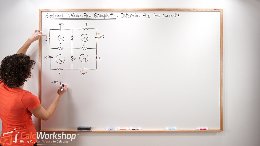
Electrical Network Flow and Kirchhoff’s Voltage Law

Then we will look at two examples of Electrical Network Flow. An electrical circuit consists of points called junctions, or nodes, with lines or arcs called branches connecting some or all of the junctions. We will look at:

• Kirchhoff’s Voltage Law

This law states that around any loop in a circuit, the voltage rises must equal the voltage drops. This ensures that by the time a charge makes it to the end of a circuit, it must have given all its energy to do work.

Linear Difference Equations and Population Movement

Lastly, we will look at the Linear Difference Equation or Recurrence Relation and how it applies to population movement or migration patterns. This linear system allows us to model a dynamic system that changes over time mathematically.

This type of study will allow us to:

• Track the movements of commodities and people groups
• Assist law enforcement in tracking criminals

Key Features of Difference Equations: All difference equations feature measured time intervals. For example,
\(\overrightarrow{x_{0}}=\) initial value,
\(\overrightarrow{x_{1}}=\) one year later,
\(\overrightarrow{x_{2}}=\) two years later
\(\ldots \overrightarrow{x_{k}}=k\) th year.

Thus, we can determine migration and movement by creating a matrix \(\mathrm{A}\) such that.

\begin{align*}
\begin{gathered}
\overrightarrow{x_{1}}=A \overrightarrow{x_{0}} \\
\overrightarrow{x_{2}}=A \overrightarrow{x_{1}} \\
\vdots \\
\overrightarrow{x_{k}}=A \overrightarrow{x_{k-1}}
\end{gathered}
\end{align*}

And the key to solving these types of problems is to find matrix A, which we will call the migration matrix (M).

For example, suppose 5% of a city’s population moves to the surrounding suburbs each year, and about \(4 \%\) of the suburban population moves into the city. In 2000, there were 600,000 residents in the city and 400,000 in the suburbs. Ignoring other factors that might influence population sizes, estimate the population in the city and the suburbs three years later, in 2003.

First, let’s identify our initial value: \(\overrightarrow{x_{0}}=\left[\begin{array}{c}\text { city } \\ \text { suburb }\end{array}\right]=\left[\begin{array}{c}600,000 \\ 400,000\end{array}\right]\)

\begin{equation}
\begin{array}{|c|c|c|}
\hline & \text { City } & \text { Suburbs } \\
\hline \text { City } & \begin{array}{l}
\text { Lives in city and } \\
\text { stays in city }
\end{array} & \begin{array}{l}
\text { Moves from } \\
\text { suburbs to city }
\end{array} \\
\hline \text { Suburbs } & \begin{array}{l}
\text { Moves from city} \\
\text { to suburbs }
\end{array} & \begin{array}{l}
\text { Lives in suburbs } \\
\text { and stays suburb }
\end{array} \\
\hline
\end{array}
\end{equation}

Next, let’s create a migration matrix where we see how the population changes, recognizing that each column must remain stochastic (total of 1 ).

\begin{align*}
M=\left[\begin{array}{ll}
0.95 & 0.04 \\
0.05 & 0.96
\end{array}\right]
\end{align*}

Now, we need to apply our migration matrix (i.e., transformation) to our initial population values and see how many people moved each year.

\(2000: \)
\begin{equation}
\overrightarrow{x_0}=\left[\begin{array}{l}
586,000 \\
414,000
\end{array}\right]
\end{equation}

\(2001: \)
\begin{aligned}
\overrightarrow{x_{1}} & =M \overrightarrow{x_{0}} \\
& =\left[\begin{array}{ll}0.95 & 0.04 \\ 0.05 & 0.96\end{array}\right]\left[\begin{array}{l}600,000 \\ 400,000\end{array}\right] \\
& =600,000\left[\begin{array}{l}0.95 \\ 0.05\end{array}\right]+400,000\left[\begin{array}{l}0.04 \\ 0.96\end{array}\right] \\
& =\left[\begin{array}{c}586,000 \\ 414,000\end{array}\right]
\end{aligned}

\(2002: \)
\begin{aligned}
\overrightarrow{x_{2}} & =M \overrightarrow{x_{1}} \\
& =\left[\begin{array}{ll}0.95 & 0.04 \\ 0.05 & 0.96\end{array}\right]\left[\begin{array}{l}586,000 \\ 414,000\end{array}\right] \\
& =\left[\begin{array}{l}573,260 \\ 426,740\end{array}\right]
\end{aligned}

\(2003: \)
\begin{aligned}
\overrightarrow{x_{3}} & =M \overrightarrow{x_{2}} \\
& =\left[\begin{array}{ll}0.95 & 0.04 \\ 0.05 & 0.96\end{array}\right]\left[\begin{array}{l}573,260 \\ 426,740\end{array}\right] \\
& =\left[\begin{array}{l}561,667 \\ 438,333\end{array}\right]
\end{aligned}

So, the population change in 2003 shows there are 561,667 people now residing in the city and 438,333 people living in the suburbs.

We will see many of these applications again in future lessons, primarily when we deal with Markov Chains, Transition Matrices, Stochastic Matrices, and Eigenvalues and Eigenvectors.

Next Steps

Okay, so now it’s time to jump into the video lesson and see the fantastic real-life applications of linear equations in linear algebra.

Video Tutorial w/ Full Lesson & Detailed Examples

Get access to all the courses and over 450 HD videos with your subscription

Monthly and Yearly Plans Available

Get My Subscription Now

Still wondering if CalcWorkshop is right for you?
Take a Tour and find out how a membership can take the struggle out of learning math.