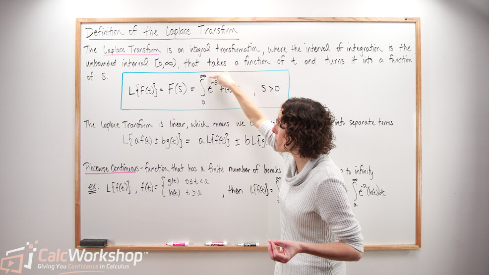
Ever wondered how to simplify “difficult” ordinary differential equations? The Laplace Transform is like a skilled translator, converting these complex equations into more approachable forms.

Jenn, Founder Calcworkshop®, 15+ Years Experience (Licensed & Certified Teacher)
Used extensively in engineering, the Laplace Transform takes a function of a positive real variable (x or t), often represented as “time,” and transforms it into a function of a complex variable, commonly called “frequency.”
Let’s jump in and see what the Laplace transform is all about!
Understanding Improper Integrals
Okay, so to better understand the Laplace transform, we must first understand the improper integral.
If
In other words, if
Convergence of Improper Integrals
Now it’s time to look at an important improper integral because it builds the foundation for what we are about to see….
If the improper integral
And this integral, if it exists, is a function of
Definition of the Laplace Transform
By definition, the Laplace transform assumes that
Basic Transforms Table
Now, computing transforms directly can be a bit complicated and tedious, so it’s by far easier to use a table of transforms to help simplify the process for us.
Keep in mind that this table isn’t exhaustive, but it does provide a solid foundation for harnessing this impressive new tool!
You might be wondering, “What is this, and how does it help solve differential equations?”
Great question! Let’s explore a few examples together to better understand its applications.
Properties of the Laplace Transform
But before we do, I want to point out two critical properties, as the Laplace transform is linear and upholds both homogeneity and superposition.
The Laplace Transform has two essential properties, linearity and superposition, which make it useful for solving complex problems:
- Linearity (Homogeneity): This means that if you multiply a function by a constant, you can just multiply the Laplace Transform of that function by the same constant.
- Superposition: This means that if you add two functions together, you can simply add their Laplace Transforms separately.
These properties make working with the Laplace Transform easier and more efficient, helping us analyze complex systems and solve differential equations in various fields like engineering, physics, and mathematics.
If
Example: Laplace Transform of a Polynomial Function
Find the Laplace transform of the function
First, we will use our first property of linearity and pull out the leading coefficient.
Next, we will notice that our function is a polynomial of the form
Easy, right?
Example: Laplace Transform w/ Exponential and Trig Functions
Find the Laplace transform of the function
First, we will use our second property and separate our two terms.
Next, we will use our table to find our transformation for the exponential function and the trigonometric function separately, as follows.
Nothing to it!
Let’s Wrap Up
Together, you’ll explore the Laplace Transform by:
- Understanding linearity and breaking up each term into separate parts.
- Discussing sufficient conditions of existence, such as piecewise continuous functions.
- Working through five detailed examples using the Definition of the Laplace Transform, Improper Integrals, and Integration by Parts.
- Creating a table of Basic Transforms and applying them to seven more examples.
Let’s go!
Video Tutorial w/ Full Lesson & Detailed Examples

Get access to all the courses and over 450 HD videos with your subscription
Monthly and Yearly Plans Available
Still wondering if CalcWorkshop is right for you?
Take a Tour and find out how a membership can take the struggle out of learning math.