Let’s expand our knowledge for discrete random variables and discuss joint probability distributions where you have two or more discrete variables to consider.

Jenn, Founder Calcworkshop®, 15+ Years Experience (Licensed & Certified Teacher)
Now is there ever a time when it is desirable to record the outcomes of several random variables simultaneously?
Sure!
Here are just a few instances:
- What about when someone studies the likelihood of success in college based on SAT scores?
- Or the rapidness and volume of a chemical gas that is released in order to determine spread and potency?
- Or the day of the year and the average temperature?
Each of these examples contains two random variables, and our interest lies in how they are related to each other.
In this chapter, we will expand our knowledge from one random variable to two random variables by first looking at the concepts and theory behind discrete random variables and then extending it to continuous random variables.
If X and Y are two random variables, then the probability of their simultaneous occurrence can be represented as a function called a Joint Probability Distribution or Bivariate Distribution as noted by Saint Mary’s College.
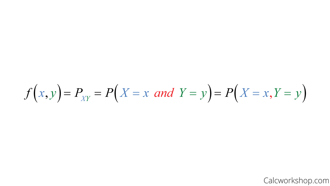
Joint Probability Formula For Discrete
In other words, the values give the probability that outcomes X and Y occur at the same time.
So, if X and Y are discrete random variables, the joint probability function’s properties are:

Joint PMF Properties
It is important to note is that we use the term probability mass function, or pmf, to describe discrete probability distributions. Whereas we use the term probability density function, or pdf, to describe continuous probability. And while there is technically a distinction between the two, you will find that they are considered synonymous and sometimes used interchangeably.
So how do we find a joint probability function and use it to find the probability?
The easiest way to organize a joint pmf is to create a table. Each cell represents the joint probability (i.e., the likelihood of both X and Y occurring at the same time).
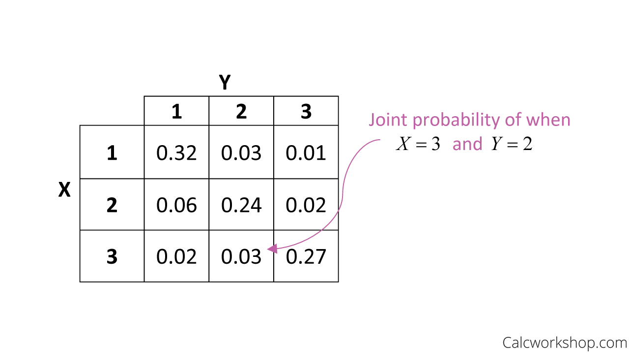
Joint Probability Table Example
Another important concept that we want to look at is the idea of marginal distributions.
The marginals of X alone and Y alone are:

Marginal Distribution Formula For Discrete
So, for discrete random variables, the marginals are simply the marginal sum of the respective columns and rows when the values of the joint probability function are displayed in a table.
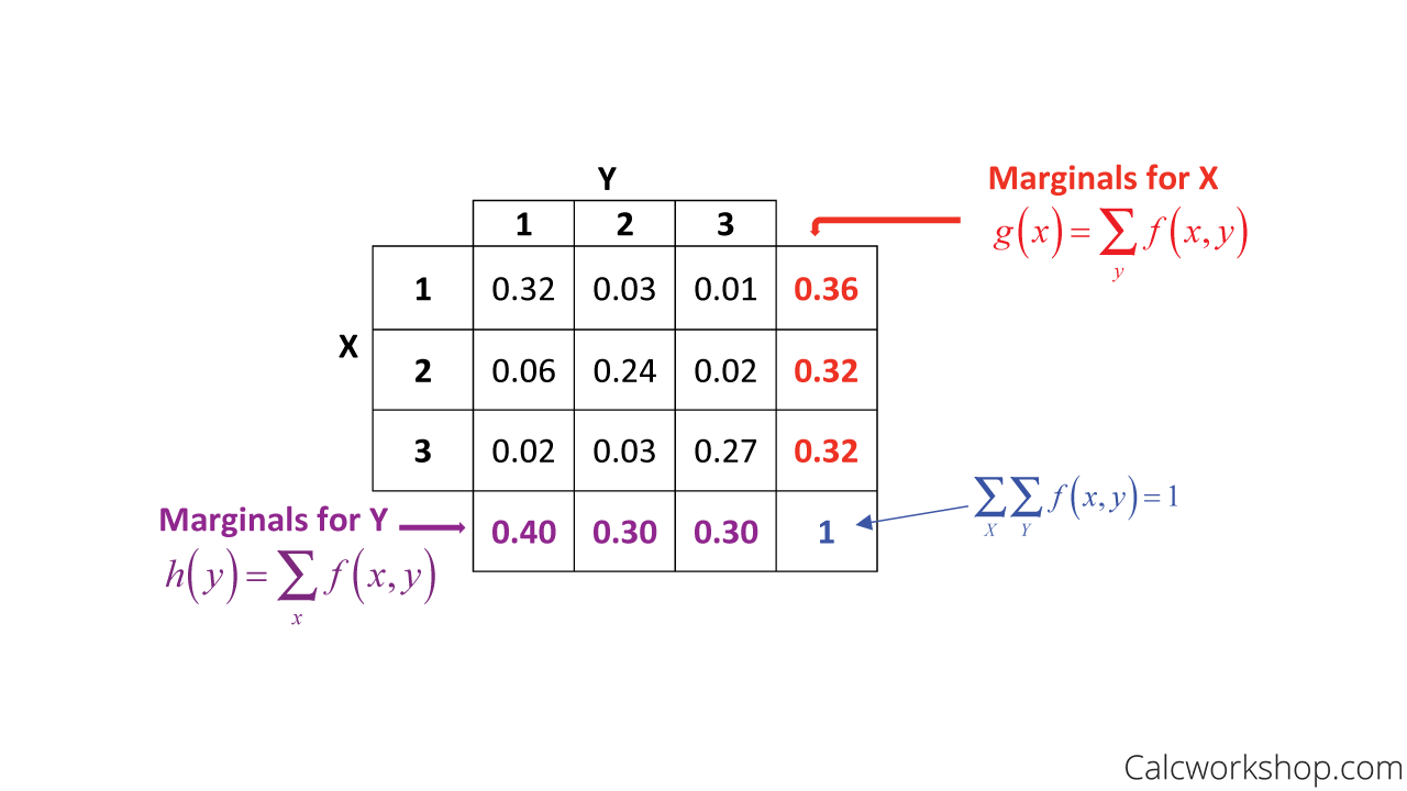
Joint And Marginal Probability Table
For example, using our table above, the marginal distributions are written as follows.
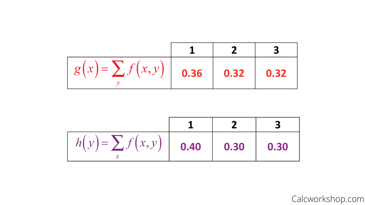
How To Find Marginal Distribution From Joint Distribution
Moreover, we can find the expected values for X and Y and the predicted value of XY.
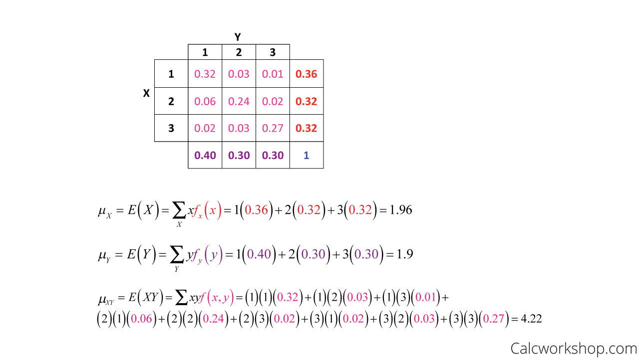
Expected Value Of XY For Discrete
Additionally, we can even use a joint probability function to find the conditional probability. This is done by restricting our focus to either a row or column of the probability table.
Together, we will learn how to create a joint probability mass function and find probability, marginal probability, conditional probability, and mean and variance.
Joint Discrete Random Variables – Lesson & Examples (Video)
1 hr 42 min
- Introduction to Video: Joint Probability for Discrete Random Variables
- 00:00:44 – Overview and formulas of Joint Probability for Discrete Random Variables
- Exclusive Content for Members Only
- 00:06:57 – Consider the joint probability mass function and find the probability (Example #1)
- 00:17:05 – Create a joint distribution, marginal distribution, mean and variance, probability, and determine independence (Example #2)
- 00:48:51 – Create a joint pmf and determine mean, conditional distributions and probability (Example #3)
- 01:06:09 – Determine the distribution and marginals and find probability (Example #4)
- 01:21:28 – Determine likelihood for travel routes and time between cities (Example #5)
- 01:33:39 – Find the pmf, distribution, and desired probability using the multivariate hypergeometric random variable (Example #6)
- Practice Problems with Step-by-Step Solutions
- Chapter Tests with Video Solutions
Get access to all the courses and over 450 HD videos with your subscription
Monthly and Yearly Plans Available
Still wondering if CalcWorkshop is right for you?
Take a Tour and find out how a membership can take the struggle out of learning math.