When you think of “differential equation,” what pops into your head?

Jenn, Founder Calcworkshop®, 15+ Years Experience (Licensed & Certified Teacher)
Calculus? Derivatives? Integrals? Fear?
I hope you’re considering the first three, and not the last one! Differential equations and their study are not only intriguing and adaptable but also incredibly useful.
What is an Ordinary Differential Equation?
At its core, a differential equation is simply an equation composed of one or more unknown functions (dependent variables) related to one or more independent variables.
In simpler terms, a differential equation (DE) includes one or more derivatives.
Easy, right?
Indeed! But as we delve deeper, we’ll see that the type, order, and linearity of a differential equation play a crucial role in how we solve and analyze them. That’s why it’s vital for us to learn how to classify these guys!
Types of Differential Equations: ODEs vs. PDEs
First, let’s talk about type.
There are two types of differential equations:
- Ordinary differential equation (ODE)
- Partial differential equations (PDE)
An ODE is a function containing only ordinary derivatives of one or more function with respect to a single variable, whereas a PDE is an equation involving partial derivatives which contain two or more independent variables.
\begin{equation}
\begin{array}{c|c}
\text { Ordinary Differential Equation } & \text { Partial Differential Equations } \\
\hline \frac{d y}{d x}-y=2 x & \frac{\partial^2 u}{\partial x^2}=\frac{\partial u}{\partial x}-\frac{\partial u}{\partial y} \\
y^{\prime \prime}+3 y^{\prime}+6 y=e^x & f_x+f_{x y}+f_y=0
\end{array}
\end{equation}
This lesson, and the remainder of this course, will deal with Ordinary Differential Equations.
Classification by Order
Alright, so now let’s talk about order.
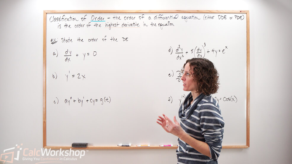
The order of a differential equation is the order of the highest derivative that appears in the equation.
Example: Defining Order
For example, let’s look at the following differential equation \(\left(\frac{d^3 y}{d x^3}\right)^2+\left(\frac{d^2 y}{d x^2}\right)^4-5\left(\frac{d y}{d x}\right)^3=4 y\) and identify all the derivatives we see
\begin{equation}
\underbrace{\left(\frac{d^3 y}{d x^3}\right)^2}_{\substack{\text { third } \\
\text { order }}}+\underbrace{\left(\frac{d^2 y}{d x^2}\right)^4}_{\begin{array}{c}
\text { second } \\
\text { order }
\end{array}}-5 \underbrace{\left(\frac{d y}{d x}\right)^3}_{\begin{array}{c}
\text { first } \\
\text { order }
\end{array}}=4 y
\end{equation}
Which one is the biggest?
Well, the biggest derivative in our equation is \(\frac{d^{3} y}{d x^{3}}\), therefore we will classify the order of the equation as “third order.”
Notice how we didn’t pay attention to the exponent, but solely on the derivative itself to classify its order.
Example: Classification
Let’s look at a few more examples, so we can get the hang of it.
Classify the order for each ordinary differential equation seen below
\begin{align*}
\begin{array}{ll}
\frac{d y}{d x}+5 y=0 \quad \rightarrow \text { first order } \\
\frac{d^{2} y}{d x^{2}}+5 \frac{d y}{d x}-3 x=0 & \rightarrow \text { second order } \\
y^{\prime \prime \prime}+\left(5 y^{\prime}\right)^{2}-3 t=2 t & \rightarrow \text { third order } \\
2 t=y-3 y^{\prime \prime}+y^{(4)}-y^{(5)} & \rightarrow \text { fifth order }
\end{array}
\end{align*}
Classification by Linearity
Now it’s time to turn our attention to classification by linearity.
An nth order ordinary differential equation \(F\left(t, y, y^{\prime}, y^{\prime \prime}, \ldots, y^{(n)}\right)=0\) is said to be linear if \(\mathrm{F}\) is linear in the variables \(y, y^{\prime}, y^{\prime \prime}, \ldots, y^{(n)}\).
Thus, an ordinary differential equation is linear if and only if it can be written in the form:
- \(a_{n}(t) \frac{d^{(n)} y}{d t^{n}}+a_{n-1}(t) \frac{d^{(n-1)} y}{d t^{n-1}}+\cdots+a_{1}(t) \frac{d y}{d t}+a_{0}(t) y=g(t)\)
And nonlinear ordinary differential equations are ones that are not linear.
But what does this really mean?
- First, the dependent variable \(y\), and all its derivatives \(y^{\prime}, y^{\prime \prime}, \ldots, y^{(n)}\) are of the first degree (i.e., the power of each term is 1 ).
- Second, the coefficients \(a_{0}, a_{1}, \ldots, a_{n}\) depend at most on the independent variable \(t\) or \(\mathrm{x}\).
- Thirdly, the dependent variable y must be a linear function.
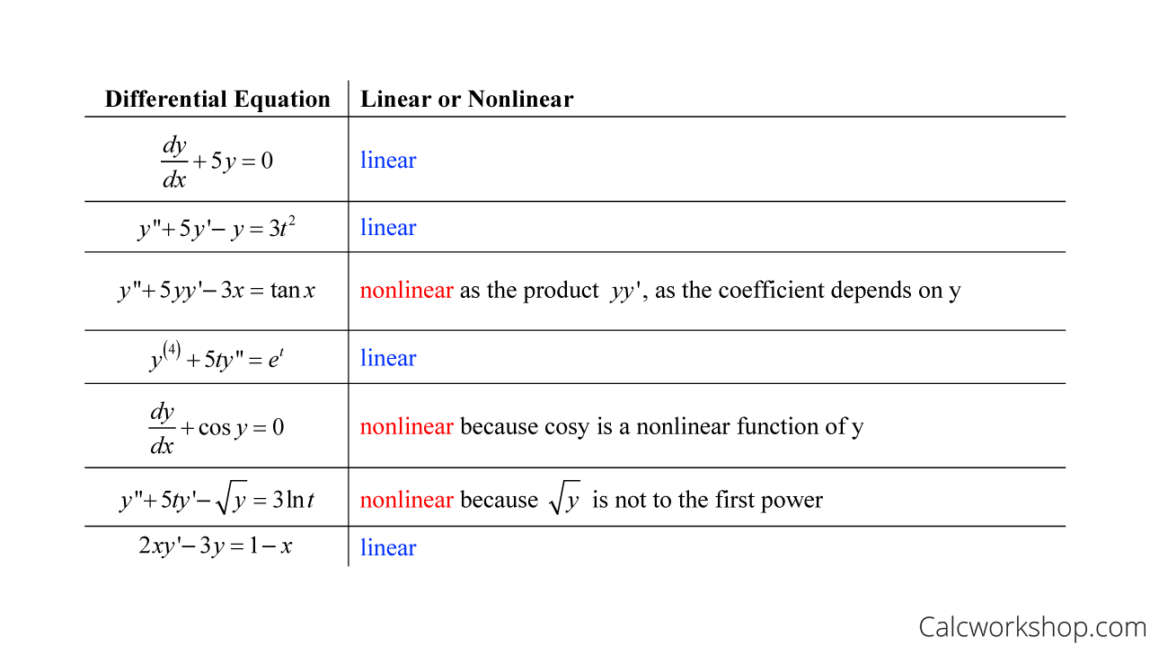
Example: Linear vs Nonlinear
For example, let’s determine whether the equations below are linear or non-linear.

Linear Nonlinear Examples
Understanding Solutions: Implicit and Explicit Functions
Our primary goal is to find the solution or solutions of an ordinary differential equation. To do this, we need to understand the difference between implicit and explicit functions.
An explicit function is an equation written in terms of the independent variable, while an implicit function is written in terms of both dependent and independent variables.

Explicit Vs. Implicit
Observe how all the explicit functions are solved for one variable (i.e., one variable on the left-hand side and every other term on the right), while the implicit functions have the variables intermixed on both sides of the equation.
We will encounter both implicit and explicit solutions throughout our study of ordinary differential equations.
Verifying Solutions of Ordinary Differential Equations
To effectively verify solutions of ordinary differential equations, it is crucial to understand the concept of “solution” in the context of the equation’s interval.
A function defined on an interval I and possessing at least n derivatives that are continuous on I, which when substituted into an nth-order ordinary differential equation reduces the equation to an identity, is said to be a solution of the equation on the interval.
In simpler terms, a solution is valid on either an open or closed interval.
Therefore, when verifying the existence of a solution, the interval of existence, sometimes referred to as the domain of the solution, must be considered.
Example: Verifying ODE Solutions
The definition above makes so much more sense when you see it in action, so let’s look at an example.
Verify that the indicated function is a solution of the given differential equation.
\begin{equation}
\color{blue}{y^{\prime \prime}} \color{black}{-} \color{black}{2 \color{red}y^{\prime}} \color{black}{+} \color{green}{y} \color{black}{=} \color{black}{0,} \color{purple}{y} \color{black}{=} \color{purple}{t e^t} \text { on the interval }(-\infty, \infty)
\end{equation}First, we take our solution \(y=t e^{t}\) and find the necessary derivatives to match the order of our differential equation
\begin{align*}
\begin{aligned}
& \color{purple}{y} \color{black}{=} \color{purple}{t e^{t}} \\
& \color{red}{y^{\prime}} \color{black}{=} \color{red}{e^{t}(t+1)} \\
& \color{blue}{y^{\prime \prime}} \color{black}{=} \color{blue}{e^{t}(t+2)}
\end{aligned}
\end{align*}Now we will substitute our functions into the differential equation and verify that the left-hand side equals the right-hand side.
\begin{align*}
\begin{aligned}
& \color{blue}{y^{\prime \prime}} \color{black}{-} \color{black}{2 \color{red}y^{\prime}} \color{black}{+} \color{green}{y} \color{black}{=} \color{black}{0} \\
& \color{black}{[}\color{blue}{e^{t}(t+2)}\color{black}{]} \color{black}{-} \color{black}{2}\color{black}{[}\color{red}{e^{t}(t+1)}\color{black}{]} \color{black}{+} \color{black}{[}\color{green}{t e^{t}}\color{black}{]} \color{black}{=} \color{black}{0} \\
& \color{black}{[}\color{blue}{t e^{t}+2 e^{t}}\color{black}{]} \color{black}{-} \color{black}{2}\color{black}{[}\color{red}{t e^{t}+e^{t}}\color{black}{]} \color{black}{+} \color{black}{[}\color{green}{t e^{t}}\color{black}{]} \color{black}{=} \color{black}{0} \\
& t e^t+2 e^t-2 t e^t-2 e^t+t e^t=0 \\
& 2 t e^t+2 e^t-2 t e^t-2 e^t=0 \\
& 0=0
\end{aligned}
\end{align*}
And that’s all there is to verifying a solution. Easy, right?
Wrapping Up
In this lesson, you will:
- Learn to classify differential equations in terms of type, order, and linearity
- Verify explicit and implicit solutions
- Get introduced to the notion of one-parameter and n-parameter family of solutions
- Explore particular solutions
With this knowledge, you’ll gain a deeper understanding of differential equations and their applications.
It’s going to be fun, so let’s get after it!
Video Tutorial w/ Full Lesson & Detailed Examples

Boost Your Calculus Scores with Step-by-Step Instruction
Jenn’s Calculus Program is your pathway to confidence. Each lesson tackles problems step-by-step, ensuring you understand every concept.
No more knowledge gaps – Jenn’s instruction bridges the missing pieces, so you’re always in stride with your class.
Calculus won’t block your academic or professional goals. Lay a solid foundation, one lesson at a time.
Your path to calculus success is just one click away.
Get access to all the courses and over 450 HD videos with your subscription
Monthly and Yearly Plans Available
Still wondering if CalcWorkshop is right for you?
Take a Tour and find out how a membership can take the struggle out of learning math.