Understanding Riemann Sums (Your First Step In Integral Calculus)

Have you ever felt the desire to “UNDO” something?

Jenn (B.S., M.Ed.) of Calcworkshop® teaching riemann sum

Jenn, Founder Calcworkshop^®, 15+ Years Experience (Licensed & Certified Teacher)

Consider how in math, every action has a REVERSE.

For example, subtraction is the “UNDO” for addition, and division is the REVERSE for multiplication.

Square roots “UNDO” squares, and logarithms REVERSE exponentials.

This concept continues in calculus with anti-differentiation reversing differentiation.

What’s that?

Well, it’s the antiderivative or, as I like to say, “the derivative in reverse” or “backwards derivatives.”

Isn’t it interesting how math consistently offers a way to backtrack? Much like that CTRL-Z shortcut on your keyboard (CMD-Z for you Mac Folks)

In other words, Anti-Differentiation is like CTRL-Z(ing) the derivative to return to the original function!

Your Key Concepts:

Antidifferentiation:

Antidifferentiation is reversing differentiation.
It means finding the original function when we know its rate of change. Put simply, if $f (x)$ shows how fast something changes.
Then its antiderivative $F (x)$ tells us the state (position) of that thing after some time, plus a constant $C$ since we might not know the starting point.

Riemann Sums:

Riemann sums are a way to guess the area under a curve by breaking it into simple shapes like rectangles or trapezoids.
The more shapes we use, the closer we reach the true area.
Different rules, like the Left Endpoint Rule or Midpoint Rule, guide us in estimating how big these shapes should be to mimic the curve’s shape.

Definite Integration:

Definite integration is about finding the precise area under a curve from point $a$ to point $b$ .
It refines the Riemann sums to the point where the rectangles (or other shapes) are infinitely thin, giving the exact result.
Mathematically, it calculates $F (b) - F (a)$ , the difference in the antiderivative $F (x)$ at the end and the start of the interval, which equals this exact area.

Now let’s learn more about each of these ideas…

Integration: The Smoother Way to Say “Anti differentiation”

But antidifferentiation and antiderivative are quite a mouthful to say, don’t you think?

Thankfully, another way of saying antidifferentiation is to say Indefinite Integration, or more simply, integration.

Before we go any further, we need to talk about two types of integration:

Indefinite
Definite

Indefinite Integration helps us to find the family of functions F(x) when we are given its derivative f(x).

$\int f (x) d x = F (x) + C$

Definite Integration is the process of finding a numerical value that represents the area under a curve over an interval [a,b].

Also known as the Riemann Integral.

$\int_{a}^{b} f (x) d x = F (b) - F (a)$

Next, we’ll explore how Riemann Integration works to give us these precise numbers.

Integration: The Tool for Area Measurement

One of the most useful things that integration does for us, besides undoing the derivative, is to calculate the area of a plane region!

In other words, it calculates the area under the curve!

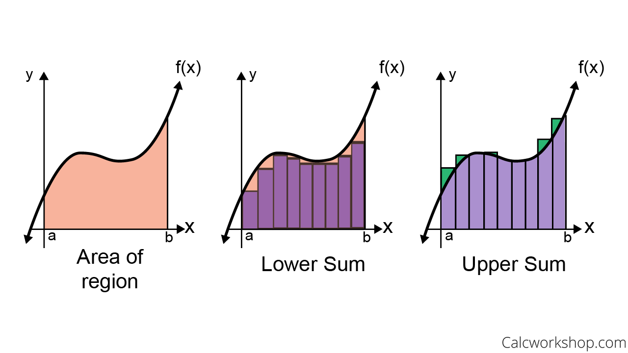
Bernhard Riemann, a pioneering German mathematician, found an ingenious way to estimate the area under curves. He did this by breaking the area down into rectangles and tallying up their individual areas.

And then comes the ingenious twist!

If we divide the region into an infinite number of rectangles, such that the width of each rectangle is infinitesimally small, then the sum of these itty-bitty rectangular areas will equal the area of the plane region!

The approximation of the area under a curve is called a Riemann Sum.

Finding Areas and Distances

How Riemann Sums Help Us Measure Area

Let’s look at the notation you will utilize for Riemann Sums.

It’s straightforward, really: the area of a rectangle is just its width multiplied by its height.

So, if $Δ x$ represents the width of each rectangle in our approximation and $f (x)$ is the height, then multiplying these together gives us the area of one rectangle, $Δ x f (x)$ .

Thus, if we wish to estimate the area of a region, we will subdivide the region into a specified number of rectangles, $n$ , such that.

$\sum_{i = 0}^{n} (Δ x) (f (x_{i}))$

And this formula is called the Riemann Sum Approximation, which we will use to estimate the area under the curve.

✏️ Take note, though, there are a few ways to calculate this:

Right Endpoint
Left Endpoint
Midpoint Rule
Trapezoidal Rule

Technically, the Trapezoid Rule and its more advanced cousin, Simpson’s Rule, are not Riemann sum approximations.

But because their approximation and approach are strikingly similar to a Riemann Sum, we will learn how to wield their power along with the other estimations.

Riemann Sums: Calculating Areas Step by Step

How do we put Riemann Sums to practical use?

Imagine we have a curve defined by $f (x)$ within the interval [a,b].

Our goal is to subdivide the interval (region) into $n$ rectangles (or trapezoids if we’re using that approach) and then calculate the area using one of four methods:

Left
Right
Midpoint
Trapezoidal

Here is the straightforward, three-step process:

Determine the width ( $Δ x$ ) of each rectangle with the formula:

$Δ x = \frac{b - a}{n}$

Select a method to calculate the area, rectangle or trapezoid:

\begin{aligned} Area Rectangle = (width) (height) \\ Area Trapezoid = \frac{1}{2} (base) (h_{1} + h_{2}) \end{aligned}

Insert the appropriate height values $f (x_{i})$ into our chosen method and perform the calculation.

Let’s look at an example.

Example: Approximations using Rectangular and Trapezoidal Areas

Estimate $\int_{1}^{7} x^{2} d x$ using:

Left Endpoint Riemann Sum
Right Endpoint Riemann Sum
Midpoint Rule
Trapezoidal Approximation

with three equal subintervals.

Let’s take a moment to identify the important components of the integral expression.

If $\int_{1}^{7} x^{2} d x$ :

Then the curve is $f (x) = x^{2}$ .
And the closed interval [a,b] is [1,7].

Step 1: Determine the Width

Our width, $Δ x$ , is found by:

$Δ x = \frac{b - a}{n}$

$Δ x = \frac{7 - 1}{3} = \frac{6}{3} = 2 .$

This means that each rectangle or trapezoid will have a width of 2.

Step 2: Applying Approximation Formulas

Next, we’ll use our approximation methods:

For the left endpoint, we calculate are to be: 70

left riemann sum calculation and area under the curve

Notice how the function $f (x)$ is increasing over the interval.

This means that the left Riemann sum is a lower estimation as the rectangles we created are below (under) the curve.

For the right endpoint, it comes out to: 166

right riemann sum calculation and area under the curve

Because $f (x)$ is increasing, the right Riemann sums is an overestimation of the area as the rectangles are above the curve.

Using the midpoint of subintervals we get: 112

midpoint rule calculation and area under the curve

Notice how the rectangles are both under and over the curve $f (x)$ .

This indicates that the midpoint rule is a much better indicator for approximating the true area under the curve.

And with trapezoids, we calculate the area to be: 118

trapezoidal approximation calculation and area under the curve

Since the function $f (x)$ is increasing and concave up, the trapezoidal rule will yield a slightly higher estimation to the true area of the curve.

But it is important to note that the trapezoidal rule, along with the midpoint rule, are the most accurate estimates for approximating the area under the curve.

In general:

For a concave-up function:

The left Riemann sum and midpoint rule underestimate the area.
The right Riemann sum and trapezoidal rule overestimate the area.

For a concave-down function:

The right Riemann sum and trapezoidal rule underestimate the area.
The left Riemann sum and midpoint rule overestimate the area.”

It is always important to check whether a function is increasing or decreasing and its concavity to determine whether an estimation is an over or under approximation.

Isn’t math fascinating? These different approaches shed light on the beauty of approximations!

Video Tutorial w/ Full Lesson & Detailed Examples (Video)

calcworkshop jenn teaching definition derivative

Boost Your Calculus Scores with Step-by-Step Instruction

Jenn’s Calculus Program is your pathway to confidence. Each lesson tackles problems step-by-step, ensuring you understand every concept.

No more knowledge gaps – Jenn’s instruction bridges the missing pieces, so you’re always in stride with your class.

Calculus won’t block your academic or professional goals. Lay a solid foundation, one lesson at a time.

Your path to calculus success is just one click away.

Get access to all the courses and over 450 HD videos with your subscription

Monthly and Yearly Plans Available

Improve My Grade! Subscribe Now

Still wondering if CalcWorkshop is right for you?
Take a Tour and find out how a membership can take the struggle out of learning math.

4.9 / 5

1,128 Reviews

Kevin S.10-30-24 - CO, United States

I had never even heard of discrete math before I had to take it for my Bachelor's in Cybersecurity. I had actually hoped that my math days were done! I suffered through class not understanding any of the presentations until I stumbled across Calcworkshop. I used the Calcworkshop lessons more than I used my instructor's lectures and my book. I ended up with a high B (just 12 points away from an A) thanks to Jenn. Without her easy to understand style of teaching, I'm not sure I would have even passed the class. Thank you so much!!!

Richard10-29-24 - Norway

Very well structured and site. It is well structured giving a good overview of the different topics regarding all mathematics where you easily can choose which path is applicable to your specific needs.The video lectures are superb with introduction to the topic followed by a detailed theoretically explaination and what I personally get most out of is; heaps of examples where you are taken and shown, step by step, the prosess of solving the problem. They also includd practice sheets and solutions to test yourself after each chapter. There is a lot to undertake on this site, but it provides an easy and understandable interface to map out what you need to do. The site has been very helpfull for me and I highly recommend it.

RobWP10-26-24 - United States

I am taking this course for mainly linear algebra review. It is a course that I have had but fairly long ago. I'm currently working in masters in data science and linear algebra namely transformations is something that has come up and I thought I need a good review on. I so far what I have liked about the course is, the common sense approach. Her approach makes it easy to remember the concepts because of her common sense approach. I like the fact that she gives information that is not really in any textbooks. I can vouch for that because not only have I used textbook recently to review I have had a formal class in the past that used textbooks. She goes over things thoroughly and for the price it's very much worth it. I have had many quarters of formal calculus and differential equations courses and I am kind of anxious to look to see what her approach to calculus is. I can't really answer how this class would be for a novice or someone who has not had linear algebra the past, but I really don't think they need to worry about that. Her method I feel will make a novice be successful and to understand the material. She is very easy to understand. Gives good examples but doesn't beat a dead horse either. What I like about her introductory remarks is that she says what linear algebra is all about and she points out what the core of the linear algebra is about and what you need to know. Having taken it before I would have to agree and she is dead on spot.

Robbin03-18-25 - CO, United States

Very well organized, helpful and comprehensive. It is great also to have access to prior course material so you can easily go back and refresh if you need to. Jenn is very clear and the number of examples leaves one comfortable with each topic. Couldn't be happier.

RCJK03-07-25 - ID, United States

I had to take Calculus I and II as accelerated classes while working full time. It was my first time taking this courses and was very overwhelming. Calcworkshop really made learning the subjects easier for me by having all the subjects easy to find and easy to understand explanations. I received a B in both classes which I am extremely happy with doing the classes in double time.

Jacqueline S.03-07-25 - SC, United States

Jenn is awesome!Her breakdown of the topic is beyond what you would expect. She is showing you how to arrive at the answer instead of doing a simple equation. Most people need to know the why it give confidence and structure to the learning process. This is what Jenn is great at, she knows how to deliver the information to a non math mind in a way that instills knowledge that you can forever draw from as you move forward. It's really well thought out. She is a true master teacher. Thanks for all that you do for us! Hugs n Blessings... JS

Rose M.03-07-25 - CA, United States

Best instructor ever, I have never had Math explained in a way that was so interesting. Her lectures and instruction is explained perfectly, and I will continue to use this for all my future math courses.

A Reviewer03-07-25 - United States

I needed help with college precalculus, they provided more than enough help that allowed me to succeed and get the scores I needed.

Jujuana03-05-25 - MO, United States

I love the videos the way each lesson is explained step by step. I love that she has examples that you can go over again and again in order to understand the way algebra works. I was lost because my instructor was flying through each lesson and I was totally lost. I attached my syllabus and they helped me stay focus on what I was working and give me a guide to go back and refresh what I went over in class.

Stacey01-31-25 - AZ, United States

Hello, I highly recommend getting a subscription to Jenn and her Calcworkshop teaching math service. I did a general, "go from bad to good at math", Google search and found out about Calcworkshop through responses to the topic on reddit. I've just started watching her videos and found them to be extremely helpful. I'm going back to college after a long absence and math was never my strong suit. So I'm starting at the very bottom of her available subjects and going from there. Just watching a couple of the videos has taken me from being dragged along not understanding to following along just fine in my math class. I'm moving from the "I'll never get this", to the "I look forward to understanding this", mindset in approaching math. This for me is huge, and even though I have a long way to go, I'm confident I will get there thanks to Jenn. Totally worth it!

Kathy W.01-14-25 - WA, United States

Calcworkshop is an outstanding source to learn math and understanding math concepts. Jenn is an outstanding master teacher. Every lesson is clearly presented making understanding easy to grasp. Practice lessons with accompanying answers are given for each section. I am 82, a retired teacher and lifelong learner. Learning calculus has always been on my bucket list. Calcworkshop is helping me reach my goal.

Cheryl01-14-25 - NY, United States

Calc workshop is the absolutely best resource for math and I have seen almost everything that exists out there. I have even recommended it to my daughter's school so that all the kids could use the videos during the summer months for the subject they plan to study in the fall. They are guaranteed to get a A if they have watched the videos and completed the problems before taking the class. Students who are weak in areas can access lower level classes and those who seek to advance above grade level can do so. The videos and exercises are crystal clear and the excellent presentations raise the bar for teachers everywhere. I have always believed that one great math teacher is important in the education process. The videos, exercises and problems are excellent. It is not possible to have ANY knowledge gaps. I have never seen anything on the market that even begins to compete with it!

Justin N.12-22-24 - OK, United States

Calculus can be a scary subject. I know I was scared. I had been out of any math class for over 23 years. I had taken an 8 week Calculus 1 class and felt like I was overloaded. Going into Calculus 2 I found CALCWORKSHOP.com. I used the training videos and material to really dive back into Calc 1 and prepare for Calc 2. Long story short with the material provided and ample study time, I finished Calc 2 with a 95%. Thanks Jenn!

Shelby12-10-24 - OH, United States

CalcWorkshop was a wonderful resource as someone going onto a college calculus 1 class after not having taken a math course in a year! Jenn always explained things in a logical order that built upon previous lessons, and the way she explained topics was always easy to understand. Calcworkshop saved this semester for me, and I couldn't be more grateful to have found this site. :)

Jordan Q.12-09-24 - AR, United States

Anyone struggling with math at any level would greatly benefit from this product. I signed up for it immediately after getting a D on my first exam in calculus 2 and ended up getting A's and B's on the remaining exams, getting a B overall in the class. Jenn breaks down the topics, without skipping any steps, in a way that makes them very easy to understand. I highly recommend this product!

N8Booker11-28-24 - MA, United States

I'm in school to get my degree Networking and Cybersecurity and I'm in my first year. I've been away from school for quite a long time so the concepts that are being taught although not foreign to me, have so much dust on them from a lack of being used in real world applications regularly.I stumbled upon CalcWorkshop by pure chance and it has been a game changer for me. Jen filled in the gaps in between what my Professor is teaching at a rapid fire pace and where my brain grasps and applies it. If not for Jen's approach, I'd have failed my test I took miserably!Am I grateful? It goes beyond words and not I recommend her workshops to everyone!

Kevin S.10-30-24 - CO, United States

Richard10-29-24 - Norway

RobWP10-26-24 - United States

RCJK03-07-25 - ID, United States

Jacqueline S.03-07-25 - SC, United States

See more reviews on Shopper Approved