Did you know that the normal distribution plays an important role in probability?

Jenn, Founder Calcworkshop®, 15+ Years Experience (Licensed & Certified Teacher)
It’s true!
Because you can find the probability of an event simply by finding the area under a normal curve.
And that’s why we’re doing a complete review of the normal distribution including how to use the empirical rule and z-scores to obtain the probabilities of an event.
Let’s go!
Did you also know that a symmetric density curve is also called a normal distribution, or a gaussian distribution?
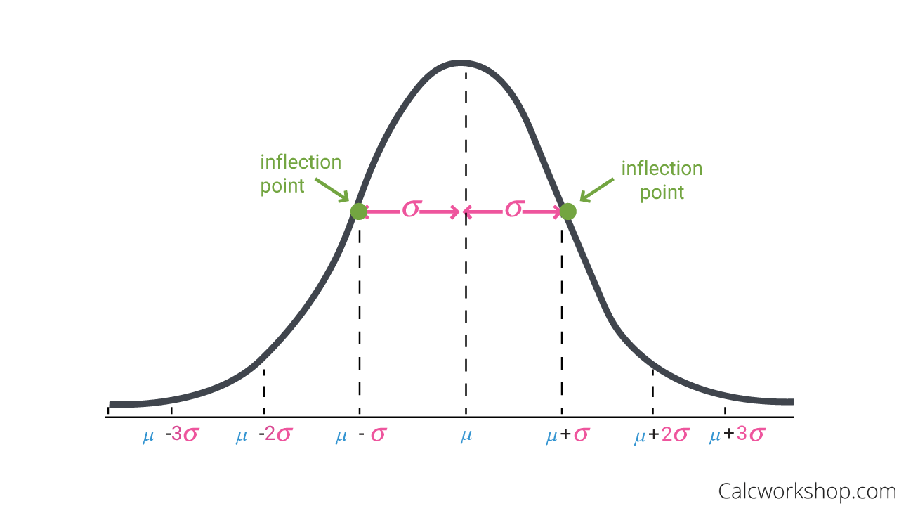
Visually, this type of distribution looks like a bell curve. The mean, median, and mode are found at the center of the distribution, and the standard deviation is the distance from the center to the change of curvature points on either side.

Normal Distribution Curve
These curvature points also referred to as inflection points, are found using our standard deviation.
The standard deviation measures how data values deviate from the mean, and behaves like a ruler, by measuring how one value compares to the whole. In other words, if we take the mean (average) and add or subtract the standard deviation, we create a normal distribution curve.
Now, our ultimate goal in analyzing any distribution is to determine the probability, or the likelihood, that an event will occur.
The density function for the Normal distribution is shown below.

Probability Distribution Formula
Sadly, this integral cannot be computed by hand.
Thankfully, there are two ways we can find what we are looking for without using integration:
- Approximate using the Empirical Rule
- Transform the data to a Standard Normal Distribution
Empirical Rule
The Empirical Rule, or the 68-95-99.7 Rule, uses the fact that in a normal distribution the data tends to be around one central value, where the spread has symmetry around the mean, such that 50% of the data falls to the left and 50% of the data falls to the right of the center.
More importantly, we can use our knowledge of standard deviation and recognize that:
- Approximately 68% of the observations fall within just one standard deviation of the mean.
- 95% of the observations fall within two standard deviations of the mean.
- 99.7% of observations fall within three standard deviations of the mean.
Hence, the 68-95-99.7 rule.
And using these values, we can quickly determine the likelihood that an observation will fall within one, two, or three standard deviations from the mean also noted by Statistics by Jim.
Example
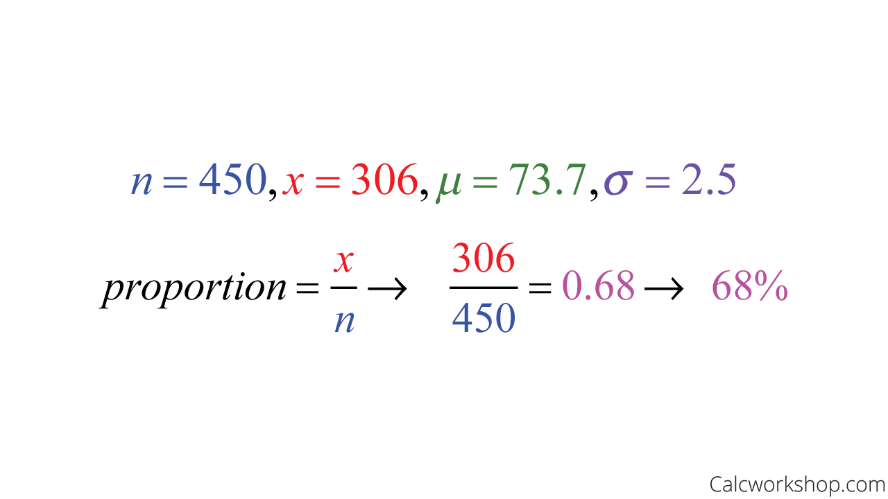
Suppose a set of 450 test scores has a symmetric, normal distribution. If the mean is 73.7 and standard deviation 2.5, determine an interval that contains approximately 306 scores.
This tells us that we are looking for an interval that contains 68% of the test scores.

Solving A Proportion
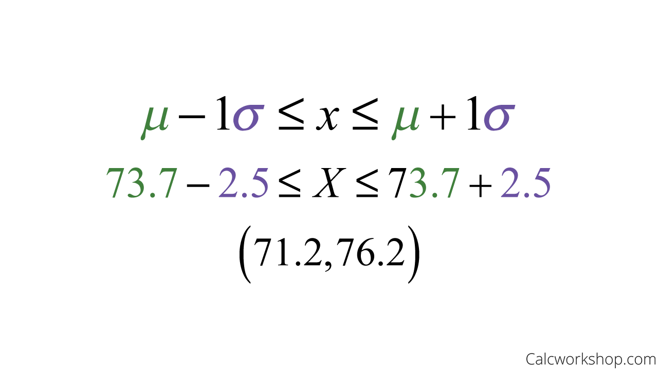
Therefore, approximately 306 scores will fall between 71.2 and 76.2 points.

Find Probability With Mean And Standard Deviation
This means that 68% of the scores falls within one standard deviation of the mean.
While the 68-95-99.7 Rule is helpful and easy to use, it’s only an approximation.
Z Score
So, is there anything that can grant us more precision?
Yep! By standardizing our values (i.e., find z-scores), we can find an accurate probability.
Recall that the z score is used when we standardize a bell curve. First, we adjust our mean to become zero (centered around the y-axis), and z scores represent the standard score, similar to the standard deviations to the left and right of the mean.
This means that a Z-score of 1 is one standard deviation above the mean, and a z score of -1 is one standard deviation below the mean.
We can now use a z-table, also called a standard normal table, to find the area under the curve, which in turn tells us the likelihood of an event taking place!
Example
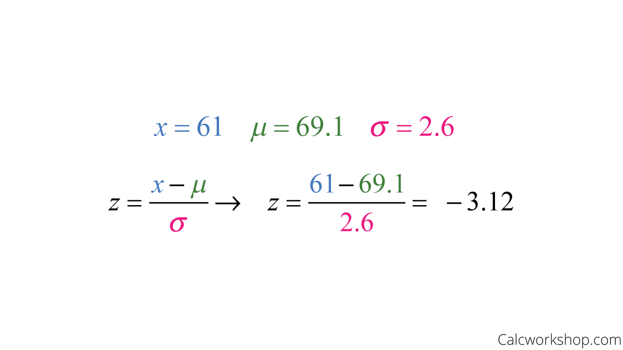
For a random sample of 428 male heights, the mean was 69.1 inches, and the standard deviation was 2.6 inches. The shortest person in the sample had a height of 61 inches.

What Does A Z Score Tell You
Because we found a z score of -3.12, this means that this particular height is more than three standard deviations below the mean. And knowing that 99.7% of observations typically fall within standard deviations of the mean, this specific height would most likely represent an outlier.
Hopefully, all of this sounds familiar, as we first introduced the concept of a normal curve and z scores back in Algebra. But don’t worry, this video lesson will help to reinforce and remind you of the fundamental concepts of the Normal Distribution and set you up for great success with finding probability in all future lessons.
Normal Distribution – Lesson & Examples (Video)
57 min
- Introduction to Video: Normal Distributions Review
- 00:00:44 – Properties of Normal Distributions and Approximating using the Empirical Rule
- Exclusive Content for Members Only
- 00:08:20 – Use the 68-95-99.7 Rule to find desired percentages (Examples #1-2)
- 00:21:05 – Standard Normal Distributions (Example #3)
- 00:40:45 – Use the standard normal distribution to find percentages (Example #4)
- 00:48:35 – Find the mean and standard deviation using the standard normal distribution and systems of equations (Example #5)
- Practice Problems with Step-by-Step Solutions
- Chapter Tests with Video Solutions
Get access to all the courses and over 450 HD videos with your subscription
Monthly and Yearly Plans Available
Still wondering if CalcWorkshop is right for you?
Take a Tour and find out how a membership can take the struggle out of learning math.