Let’s explore how predator-prey models and electrical networks can help you connect the mathematical concepts you’ve learned to real-world applications.

Jenn, Founder Calcworkshop®, 15+ Years Experience (Licensed & Certified Teacher)
By studying Lotka-Volterra equations and Kirchhoff’s Laws, you’ll uncover the hidden principles governing species interactions and electrical circuits.
And by representing and analyzing these scenarios using systems of first-order ordinary differential equations (ODEs), you’ll be empowered to:
- Tackle complex problems
- Gain a deeper understanding of the subject
Let’s go!
Lotka-Volterra Predator-Prey Model
The Lotka-Volterra predator-prey model explores how two different species interact within the same ecosystem.
If \(\mathrm{a}, \mathrm{b}, \mathrm{c}\), and \(\mathrm{d}\) are positive constants, \(\mathrm{x}\) represents the prey population and \(\mathrm{y}\) denotes the predator population, then the following system of nonlinear differential equations represent a predator-prey model:
No predators and prey population grow at a natural rate:
\begin{equation}
\frac{d x}{d t}=a x \rightarrow x=x_0 e^{a t}
\end{equation}
No prey and predator population declines at a natural rate:
\begin{equation}
\frac{d y}{d t}=-b y \rightarrow y=y_0 e^{-b t}
\end{equation}
When populations interact (Lotka-Volterra equations), the predator population increases, and the prey population decreases at a rate proportional to the frequency of interaction \(\mathrm{xy}\)
\begin{align*}
\begin{aligned}
& \frac{d x}{d t}=a x-b x y=x(a-b y) \\
& \frac{d y}{d t}=-c y+d x y=y(-c+d x)
\end{aligned}
\end{align*}
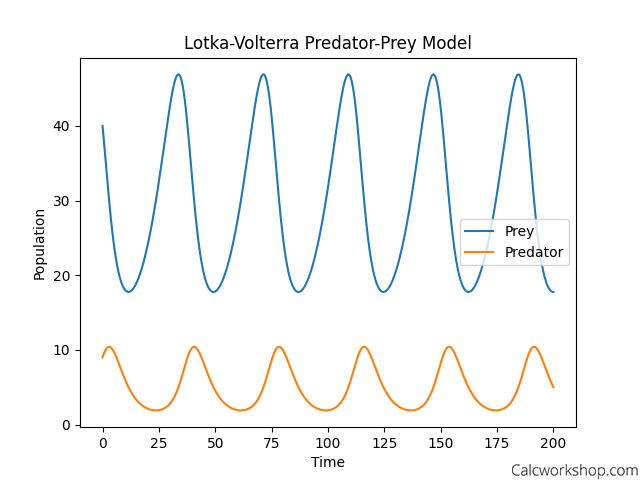
Now that we’ve discussed the Lotka-Volterra equations and their implications in predator-prey interactions let’s delve into a graphical representation of this model to better understand the underlying population dynamics.
Visualizing the Lotka-Volterra Model
In this graph, the x-axis represents time, and the y-axis represents the population size of predators and prey. The blue curve represents the prey population, while the orange curve represents the predator population.
You can observe the following:
- Oscillating populations: The populations of predators and prey oscillate over time, reflecting their interdependence.
- Impact of population growth: As the prey population increases, predators have more food, causing their population to rise. This, in turn, leads to a decline in the prey population and, eventually, the predator population.
- Model insights: The Lotka-Volterra model effectively captures the dynamics of predator-prey relationships in ecosystems, showcasing the delicate balance within these interactions.

The predator-prey population dynamics visualized using the Lotka-Volterra model, highlighting the cyclical oscillations and delicate balance within ecosystems.
Lotka-Volterra Equations and Their Applications
The Lotka-Volterra equations have far-reaching applications in economics, medicine, and biology, and they provide a valuable framework for predicting how communities coexist and interact, as the University of Tennessee nicely states.
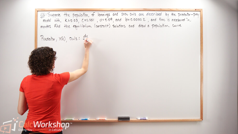
Together we will use these famous equations to analyze populations over a more extended period of time and find equilibrium (constant) solutions and population curves.
Electrical Circuits and Kirchhoff’s Law
Next, we will revisit Electrical Circuits, and use our knowledge of First-Order Differential Equations to solve a network involving Electromotive Force, Resistance, and Induction to find Current, often written as initial value problems, IVPs.
To do this, we will need the help of Kirchhoff’s Law.
An electrical circuit consists of a set of points called junctions, or nodes, with lines or arcs called branches connecting some or all of the junctions.
Kirchhoff’s Voltage Law basically says that around any loop in a circuit, the voltage rises must equal the voltage drops so that by the time a charge makes it to the end of a circuit, it must have given all its energy to do work.
So, a simple circuit containing a resistor (R), current (I), voltage (E), and inductor (L) can be represented by the following differential equation:
\begin{equation}
L \frac{d I}{d t}+R I=E(t)
\end{equation}
Visualizing the Voltage-Current Relationship in an RC Circuit
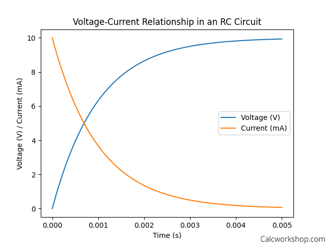
In this graph, the x-axis represents time, while the y-axis represents voltage (V) and current (mA). The blue curve illustrates the voltage across the capacitor, and the orange curve represents the current flowing through the circuit.
Observe the following:
- Initial conditions: At the start, the capacitor’s voltage is zero, and the current is at its maximum value.
- Charging process: As time progresses, the capacitor charges, causing the voltage to increase and the current to decrease, following a first-order response.
- Time constant (τ): Determined by the product of resistance (R) and capacitance (C), τ influences the charging and discharging rate of the capacitor. The graph spans 5 * τ, a common range to observe the complete process in an RC circuit.

The voltage-current relationship in an RC circuit, demonstrating the exponential charging process of a capacitor and the role of the time constant in shaping the response.
Next Steps
You’ll..
- Analyze complex networks: Apply Kirchhoff’s law to analyze electrical networks with multiple loops using simultaneous differential equations.
- Master diverse models: Dive into lessons that help you model systems of differential equations involving predator-prey and other competing models.
- Learn at your own pace: Pause, rewind, or re-watch sections to ensure full comprehension of each topic.
- Gain practical insights: Apply theories to real-world examples, tackling similar problems and challenges in your studies.
Video Tutorial w/ Full Lesson & Detailed Examples

Get access to all the courses and over 450 HD videos with your subscription
Monthly and Yearly Plans Available
Still wondering if CalcWorkshop is right for you?
Take a Tour and find out how a membership can take the struggle out of learning math.