Saddle Point
How To Find 'Em w/ Step-by-Step Examples!

Did you know that a saddle point is named for its resemblance to a riding saddle?

In fact, if we take a closer look at a horse-riding saddle, we instantly notice how the seat of the saddle is both a maximal and minimal point (i.e., minimax point).

So, that begs the question of what is a saddle point? Is it a relative extremum or something different entirely?

And how do we find the relative extrema of a surface?

Let’s find out!

As we know from single-variable calculus, extrema are the maximum or minimum values of a function.

And we determine local extrema by employing the first derivative test and second derivative test, which helps us analyze critical numbers.

Recall that a critical number of a function \(f\) is a number \(c\) in the domain such that \(f’\left( c \right) = 0\) or \(f’\left( c \right) = undefined\).

Local Maxima And Minima

Critical Points (Calculus 3)

But how does that help us find relative extrema for functions of several variables?

Well, just like in single variable calculus, to locate the relative extrema of a function of two variables, we must find critical points!

If \(f\left( {x,y} \right)\) is defined on an open region \(R\) containing \(\left( {{x_0},{y_0}} \right)\), then the point \(\left( {{x_0},{y_0}} \right)\) is a critical point of \(f\) if one of the following is true:

\begin{equation}
\begin{aligned}
&f_{x}\left(x_{0}, y_{0}\right)=0 \text { and } f_{y}\left(x_{0}, y_{0}\right)=0 \\
&f_{x}\left(x_{0}, y_{0}\right) \text { or } f_{y}\left(x_{0}, y_{0}\right) \text { does not exist }
\end{aligned}
\end{equation}

So, a critical point sometimes called a stationary point, is when the gradient vector \(\nabla f\) is zero or the points at which one of the partial derivatives does not exist.

Moreover, this also implies that the function \(f\left( {x,y} \right)\) has a horizontal tangent plane at the point \(\left( {{x_0},{y_0}} \right)\) and helps us to determine extrema.

Relative Minimum

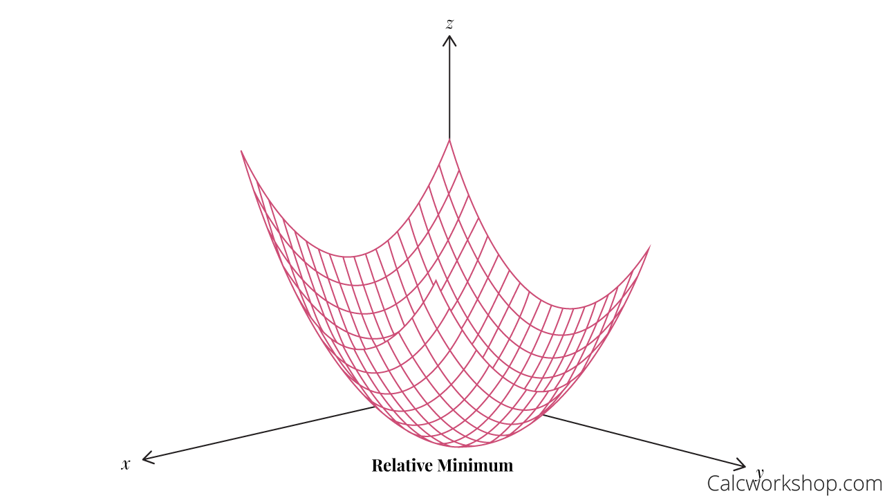
A point \(\left( {{x_0},{y_0},f\left( {{x_0},{y_0}} \right)} \right)\) is a relative minimum of a function \(f\) if there exists some region or neighborhood surrounding \(\left( {{x_0},{y_0}} \right)\) for which \(f\left( {{x_0},{y_0}} \right) \le f\left( {x,y} \right)\) for all \(\left( {x,y} \right)\) in the region.

Relative Maximum

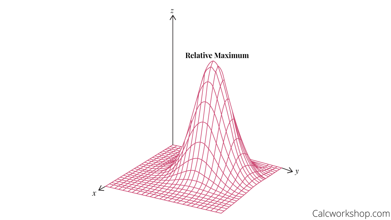
Similarly, a point \(\left( {{x_0},{y_0},f\left( {{x_0},{y_0}} \right)} \right)\) is a relative maximum of a function \(f\) if there exists some region or neighborhood surrounding \(\left( {{x_0},{y_0}} \right)\) for which \(f\left(x_{0}, y_{0}\right) \geq f(x, y)\) for all \(\left( {x,y} \right)\) in the region.

But we’re getting ahead of ourselves just a bit. Let’s first make sure we can find critical numbers of a surface.

Example – Critical Points Of Multivariable Functions

Okay, so let’s identify the critical points for the elliptic paraboloid:

\begin{equation}
f(x, y)=x^{2}+2 y^{2}-6 x+8 y+20
\end{equation}

Alright, so we begin by finding the gradient \(\nabla f\) by computing the partial derivatives with respect to \(x\) and \(y\).

\begin{equation}
f_{x}=2 x-6 \text { and } f_{y}=4 y+8
\end{equation}

Now, since both of our partials are defined for every \(x\) and \(y\) (i.e., there are no domain restrictions as both partial derivatives are polynomial functions), the critical points are those for when both first-order partial derivatives are equal to zero.

\begin{equation}
\begin{array}{cc}
f_{x}=0 & f_{y}=0 \\
2 x-6=0 & 4 y+8=0 \\
x=3 & y=-2
\end{array}
\end{equation}

Thus, we have obtained our critical point of \(\left( {3, – 2} \right)\).

Second Partials Test Theorem

Now it’s time to turn our attention to determining if our critical point is a maximum, minimum, or saddle point?

This is where our second derivative test, or second-order partial derivative test, comes into play.

Suppose \(z = f\left( {x,y} \right)\) has a critical point at \(\left(x_{0}, y_{0}\right)\) and has continuous second partial derivatives and we define a number \(D\), as \(D = {f_{xx}}\left( {{x_0},{y_0}} \right) \cdot {f_{yy}}\left( {{x_0},{y_0}} \right) – {\left( {{f_{xy}}\left( {{x_0},{y_0}} \right)} \right)^2}\), then:

• If \(D>0\) and \({f_{xx}}\left( {{x_0},{y_0}} \right)<0\) (concave down), then \(f\left( {{x_0},{y_0}} \right)\) is a relative maximum.
• If \(D>0\) and \({f_{xx}}\left( {{x_0},{y_0}} \right)>0\) (concave up), then \(f\left( {{x_0},{y_0}} \right)\) is a relative minimum.
• If \(D<0\), then \(f\left( {{x_0},{y_0}} \right)\) is a saddle point.
• If \(D=0\), the test is inconclusive, and we must examine the critical point using other means.

What Is A Saddle Point?

That’s great, but what’s a saddle point?

A saddle point is neither a local maximum nor a local minimum point.

Why?

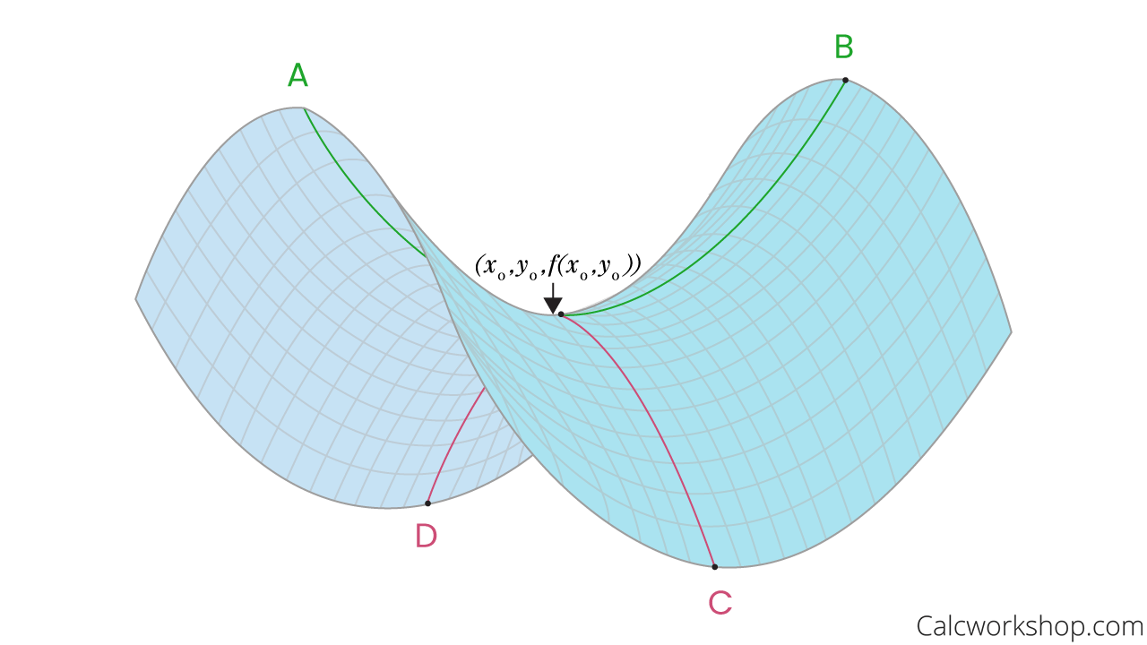
Look at the graphic below. Notice that if we draw a trace from point \(A\) to point \(B\) on the surface, our critical point \(\left( {{x_0},{y_0},f\left( {{x_0},{y_0}} \right)} \right)\) is a minimum. However, if we draw a trace from point \(C\) to point \(D\) our critical point is a maximum.

Can one point be both a minimum and a maximum simultaneously? No.

And therefore, we describe such points as saddle points as they look just like a horse saddle.

Example – Find The Local Maximum And Minimum Values And Saddle Point(s) Of The Function

Alright, so now it’s time to work through a problem.

Find all critical points for the surface \(f\left( {x,y} \right) = x{y^2} – 6{x^2} – 3{y^2}\)and determine whether each is a local maximum, minimum or saddle point.

First, we will find our first-order and second-order partial derivatives.

First Partials: \({f_x} = {y^2} – 12x\) and \(f_{y}=2 x y-6 y\)
Second Partials: \({f_{xx}} = – 12\) and \({f_{yy}} = 2x – 6\) and \({f_{xy}} = {f_{yx}} = 2y\)

Next, we will find our critical or stationary points by setting our first-order partials equal to zero.

\begin{equation}
\begin{array}{cc}
f_{x}=0 & f_{y}=0 \\
y^{2}-12 x=0 & 2 x y-6 y=0 \\
x=\frac{y^{2}}{12} &
\end{array}
\end{equation}

Now we just need to solve the system of equation by plugging our first equation into our second equation and solve.

\begin{equation}
\text { If } 2 x y-6 y=0 \text { and } x=\frac{y^{2}}{12}, \text { then }
\end{equation}

\begin{equation}
\begin{aligned}
&2\left(\frac{y^{2}}{12}\right) y-6 y=0 \\
&\frac{1}{6} y^{3}-6 y=0 \\
&y^{3}-36 y=0 \\
&y\left(y^{2}-36\right)=0 \\
&y(y+6)(y-6)=0 \\
&y=0,6,-6
\end{aligned}
\end{equation}

So, now we can resubstitute these y-values values back into our first equation to find the corresponding x-values.

\begin{equation}
\text { If } x=\frac{y^{2}}{12} \text { and } y=0, \text { then } x=0 \text { and } z=f(0,0)=0
\end{equation}

\begin{equation}
\text { If } x=\frac{y^{2}}{12} \text { and } y=6, \text { then } x=3 \text { and } z=f(3,6)=-54
\end{equation}

\begin{equation}
\text { If } x=\frac{y^{2}}{12} \text { and } y=-6, \text { then } x=3 \text { and } z=f(3,-6)=-54
\end{equation}

So, our three critical points are \(\left( {0,0,0} \right)\), \(\left( {3,6, – 54} \right)\), and \(\left( {3, – 6, – 54} \right)\)

Now it’s time to find our D-equation.

\begin{equation}
\begin{aligned}
&D=f_{x x}\left(x_{0}, y_{0}\right) \cdot f_{y y}\left(x_{0}, y_{0}\right)-\left(f_{x y}\left(x_{0}, y_{0}\right)\right)^{2} \\
&D=(-12)(2 x-6)-(2 y)^{2} \\
&D=-24 x-4 y^{2}+72
\end{aligned}
\end{equation}

Finally, apply our Second Partial Test Theorem to our three singular points and determine whether they are maximums, minimums, or saddle points.

\((0,0,0):\)
\begin{equation}
D=-24(0)-4(0)^{2}+72=72 \text { and } f_{x x}=-12
\end{equation}
\begin{equation}
\text { If } D>0 \text { and } f_{x x}<0,(0,0,0) \text { is a relative maximum }
\end{equation}

\((3,6,-54):\)
\begin{equation}
D=-24(3)-4(6)^{2}+72=-144 \text { and } f_{x x}=-12
\end{equation}
\begin{equation}
\text { Since } D<0, \text { we have a saddle point at }(3,6,-54)
\end{equation}

\((3,-6,-54):\)
\begin{equation}
D=-24(3)-4(-6)^{2}+72=-144 \text { and } f_{x x}=-12
\end{equation}
\begin{equation}
\text { Since } D<0 \text {, we have a saddle point at }(3,-6,-54)
\end{equation}

Thus, we can conclude that our surface has one relative extremum and two saddle points.

See how easy it is to determine relative extrema!

And guess what!

If we know how to find relative extrema, we also know how to optimize a surface!

It’s true.

Understanding how to identify local extrema for a function of several variables, combined with the techniques we learned for optimization problems in single variable calculus, will allow us to optimize surfaces to find such things as maximizing profit or calculating the shortest distance between points.

Together in our lesson, we will learn how to find critical (stationary) points, identify relative maximum, relative minimum, and saddle points using the second partial derivative theorem, and how to optimize a function of several variables.

Let’s get to it!

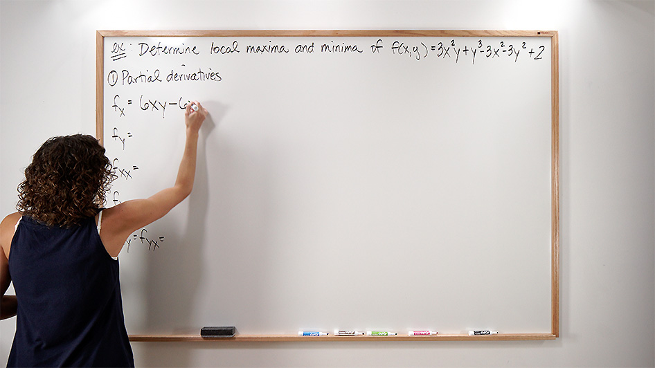
Video Tutorial w/ Full Lesson & Detailed Examples (Video)

Get access to all the courses and over 450 HD videos with your subscription

Monthly and Yearly Plans Available

Get My Subscription Now

Still wondering if CalcWorkshop is right for you?
Take a Tour and find out how a membership can take the struggle out of learning math.