Tangent Plane & Linear Approximations
w/ Step-by-Step Examples!

How to find a tangent plane?

And why would we want to?

Because of all the functions to work with, linear functions are the easiest.

So, wouldn’t it be great to treat a surface like a plane, which is a linear function in 3-space?

Good thing we can!

Equations Of Tangent Planes

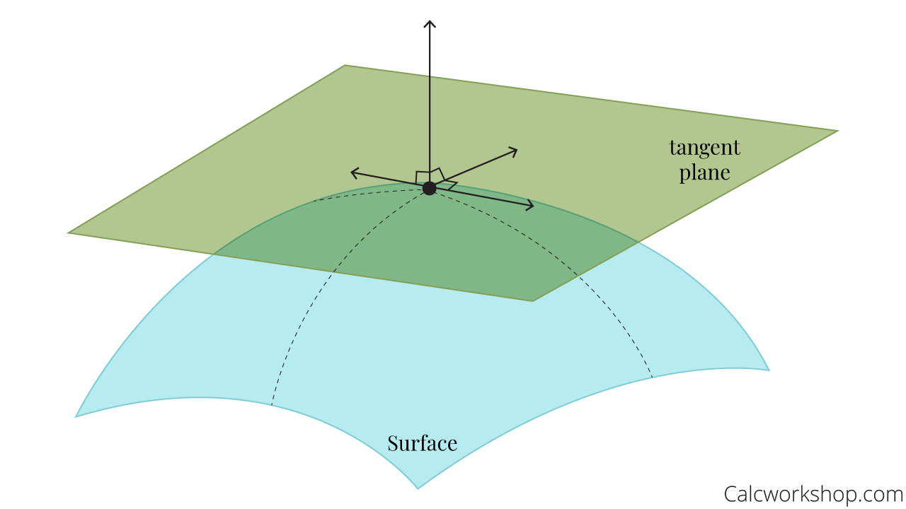
If we zoom in small enough to a point on a surface, we can approximate the function by a linear function of two variables.

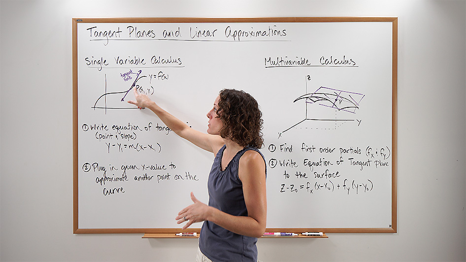
First, let’s recall that we could approximate a point by its tangent line in single variable calculus.

\begin{equation}
y-y_{0}=f^{\prime}\left(x_{0}\right)\left(x-x_{0}\right) \mathrm{x}
\end{equation}

This point-slope form of the tangent line is the linear approximation, or linearization, of \(f\left( x \right)\) at the point \(\left( {{x_0},{y_0}} \right)\).

Now, let’s extend this idea for a function of two variables.

If \(f\) has continuous first-order partial derivatives, then the equation of the tangent plane to the surface \(z = f\left( {x,y} \right)\) at the point \(\left( {{x_0},{y_0},{z_0}} \right)\) is:

\begin{equation}
z-z_{0}=f_{x}\left(x_{0}, y_{0}\right)\left(x-x_{0}\right)+f_{y}\left(x_{0}, y_{0}\right)\left(y-y_{0}\right)
\end{equation}

Which can be generalized for a linear function of two variables as:

\begin{equation}
z=A\left(x-x_{0}\right)+B\left(y-y_{0}\right)+C
\end{equation}

Where \(C = f\left( {{x_0},{y_0}} \right)\) from the point \(\left( {{x_0},{y_0},f\left( {{x_0},{y_0}} \right)} \right)\) , \(A=f_{x}\left(x_{0}, y_{0}\right)\) and \(B = {f_y}\left( {{x_0},{y_0}} \right)\).

Example

Let’s look at an example of using the formula to write a tangent plane to a surface.

Suppose we wish to find the equation of the tangent plane to the surface \(f\left( {x,y} \right) = 3{x^2}y + 2{y^2}\) at the point \(\left( {1,1} \right)\).

First, we will need to find the z-component of our point by plugging the given ordered pair into our curve.

\begin{equation}
\begin{aligned}
&z=f(x, y)=3 x^{2} y+2 y^{2} \text { at }(1,1) \\
&z=f(x, y)=3(1)^{2}(1)+2(1)^{2}=5
\end{aligned}
\end{equation}

Thus, the point on the surface is \(\left( {{x_0},{y_0},{z_0}} \right) = \left( {{x_0},{y_0},f\left( {{x_0},{y_0}} \right)} \right) = \left( {1,1,5} \right)\).

Now we have to find our partial derivatives, which are the slope of the tangent line to the surface in the x and y-direction.

\begin{equation}
f_{x}=6 x y \text { and } f_{y}=3 x^{2}+4 y
\end{equation}

Next, we substitute our ordered pair into our partial derivatives to find the instantaneous slopes.

\begin{equation}
f_{x}(1,1)=6(1)(1)=6 \text { and } f_{y}(1,1)=3(1)^{2}+4(1)=7
\end{equation}

Finally, we are ready to write the tangent plane equation at the point.

\begin{equation}
\begin{aligned}
&z-z_{0}=f_{x}\left(x_{0}, y_{0}\right)\left(x-x_{0}\right)+f_{y}\left(x_{0}, y_{0}\right)\left(y-y_{0}\right) \\
&z-5=6(x-1)+7(y-1)
\end{aligned}
\end{equation}

And its linearization is the equation:

\begin{equation}
f(x, y)=6(x-1)+7(y-1)+5
\end{equation}

Simple!

Linear Approximation In Calc 3

But here’s what’s cool.

The linear function whose graph is the tangent plane:

\begin{equation}
f(x, y)=f_{x}\left(x_{0}, y_{0}\right)\left(x-x_{0}\right)+f_{y}\left(x_{0}, y_{0}\right)\left(y-y_{0}\right)+f\left(x_{0}, y_{0}\right)
\end{equation}

is called the linearization of \(f\) at \(\left( {a,b} \right)\).

And the approximation…

\begin{equation}
f(x, y) \approx f_{x}(a, b)(x-a)+f_{y}(a, b)(y-b)+f(a, b)
\end{equation}

is called the linear approximation or the tangent plane approximation of f at \(\left( {a,b} \right)\).

Example

Alright, so if the surface \(f\left( {x,y} \right) = 3{x^2}y + 2{y^2}\) is differentiable at the point \(\left( {1,1} \right)\), then estimate \(f\left( {1.1,0.9} \right)\) by using the tangent plane approximation.

Since, we have already found the linearization of \(f\) to be \(f\left( {x,y} \right) \approx 6\left( {x – 1} \right) + 7\left( {y – 1} \right) + 5\) all we have to do is substitute our new point \((1.1,0.9)\) into the equation and simplify.

\begin{equation}
\begin{aligned}
&f(x, y) \approx 6(x-1)+7(y-1)+5 \\
&f(1.1,0.9) \approx 6(1.1-1)+7(0.9-1)+5 \\
&f(1.1,0.9) \approx 4.9
\end{aligned}
\end{equation}

Great!

Error In Linear Approximation

Remember that approximations are only useful and significant near the point where the plane is tangent. The further away from the original point you go, the worse your approximation.

Actual Vs. Approximation

For instance, let’s match the actual value to our approximated value and see how they compare.

\begin{equation}
\begin{array}{cc}
\text { Actual Value } & \text { Approximated Value } \\
f(x, y)=3 x^{2} y+2 y^{2} \text { at }(1.1,0.9) & f(x, y) \approx 6(x-1)+7(y-1)+5 \\
f(1.1,0.9)=3(1.1)^{2}(0.9)+2(0.9)^{2} & f(1.1,0.9) \approx 6(1.1-1)+7(0.9-1)+5 \\
f(1.1,0.9)=4.89 & f(1.1,0.9) \approx 4.9
\end{array}
\end{equation}

It looks like our estimation is spot on the mark!

But as you can see, with every approximation, there is always some error involved.

Therefore, a practical application of linear approximation is to estimate the error in the value of a function given estimates of error in its inputs.

Differentials

And we describe the errors in estimating as differentials.

For a function of two variables \(z = f\left( {x,y} \right)\), we define the differentials \(dx\) and \(dy\) to be independent variables and can be given any values.

Thus, the total differential \(dz\) estimates the error in \(z\) by \(dz = {f_x}\left( {{x_0},{y_0}} \right)dx + {f_y}\left( {{x_0},{y_0}} \right)dy\).

So, in the notation of differentials, the linear approximation \(f\left( {x,y} \right) \approx {f_x}\left( {a,b} \right)\left( {x – a} \right) + {f_y}\left( {a,b} \right)\left( {y – b} \right) + f\left( {a,b} \right)\) can be written as \(f\left( {x,y} \right) \approx dz + f\left( {a,b} \right)\).

Example

For example, the volume of a cylinder with radius \(r\) and height \(h\) is \(V = \pi {r^2}h\). Assume that \(r = 3\) m and \(h = 15\) m such that the volume is \(V = 135\pi \) \({m^3}\) . If the measurement of error in \(r\) and \(h\) is at most 0.05m, then estimate the error in the computed volume.

Well, let’s first identify what we’ve been given.

We know that the error (i.e., the differentials) for both the radius and height are 0.05m.

Thus.

\begin{equation}
d r=0.05 \text { and } d h=0.05
\end{equation}

And knowing our formula to estimate the total differential is \(dz = {f_x}\left( {{x_0},{y_0}} \right)dx + {f_y}\left( {{x_0},{y_0}} \right)dy\) we can adapt it to our current formula as:

\begin{equation}
d V=V_{r} d r+V_{h} d h
\end{equation}

So, that means we must now find the partial derivatives for \(r\) and h, respectively.

\begin{equation}
V_{r}=2 \pi r h \text { and } V_{h}=\pi r^{2}
\end{equation}

Next, we will substitute our given values \(r = 3\) m and \(h = 15\) m

\begin{equation}
V_{r}=2 \pi(3)(15)=90 \pi \text { and } V_{h}=\pi(3)^{2}=9 \pi
\end{equation}

Thus, when \(r = 3\) m and \(h = 15\) m and \(dr = 0.05\) and \(dh = 0.05\) , the error in V is approximately
\begin{equation}
\begin{aligned}
&d V=V_{r} d r+V_{h} d h \\
&d V=(90 \pi)(0.05)+(9 \pi)(0.05) \\
&d V=4.95 \pi \mathrm{m}^{3}
\end{aligned}
\end{equation}

Nice.

Don’t worry. We will walk through numerous examples to help make sense of this fantastic topic.

Get ready to learn how to find an equation of the tangent plane to a given surface at a specified point, find the linearization at a point, calculate the linear approximation of a function, and find the differentials of a function.

There’s a lot to unpack, so let’s get to it!

Video Tutorial w/ Full Lesson & Detailed Examples (Video)

Get access to all the courses and over 450 HD videos with your subscription

Monthly and Yearly Plans Available

Get My Subscription Now

Still wondering if CalcWorkshop is right for you?
Take a Tour and find out how a membership can take the struggle out of learning math.