Normal Approximation
w/ 5 Step-by-Step Examples!

What is normal approximation?

And how does it relate to statistics?

Let’s find out, shall we…

If certain conditions are met, then a continuous distribution can be used to approximate a discrete distribution?

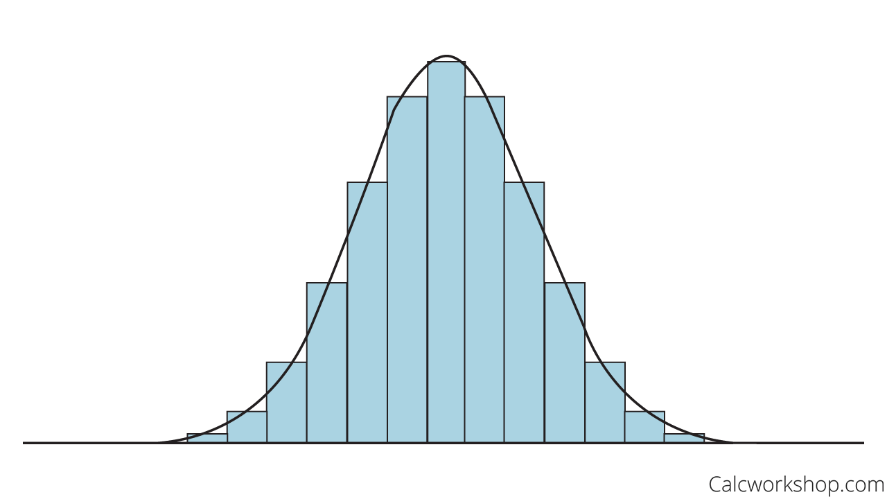
The Normal Distribution (continuous) is an excellent approximation for such discrete distributions as the Binomial and Poisson Distributions, and even the Hypergeometric Distribution.

How?

Thanks to the Central Limit Theorem and the Law of Large Numbers.

Central Limit Theorem

First, the Central Limit Theorem (CLT) states that for non-normal distribution, as the sample size increases, the distribution of the sample means becomes approximately Normal. So, as long as the sample size is large enough, the distribution looks normally distributed.

Law Of Large Numbers

Secondly, the Law of Large Numbers helps us to explain the long-run behavior. It states that if we observe more and more repetitions of any chance experiment, the proportion of times that a specific outcome occurs will approach a single value as noted by Lumen Learning.

Coin Toss Example

For example, if we flip a coin repeatedly for more than 30 times, the probability of landing on heads becomes approximately 0.5. This is why we say you have a 50-50 shot of getting heads when you flip a coin because, over the long run, the chance or probability of getting heads occurs half the time.

So, with these two essential theorems, we can say that with a large sample size of repeated trials, the closer a distribution will become normally distributed.

But why do we care?

Because for certain discrete distributions, namely the Binomial and Poisson distributions, summing large values can be tedious or not practical. Thankfully, the Normal Distribution allows us to approximate the probability of random variables that would otherwise be too difficult to calculate.

Now, before we jump into the Normal Approximation, let’s quickly review and highlight the critical aspects of the Binomial and Poisson Distributions.

Binomial Distribution

A binomial random variable represents the number of successes in a fixed number of successive identical, independent trials. Each trial has the possibility of either two outcomes:

• Success
• Or Failure

And the probability of the two outcomes remains constant for every attempt. And as the sample size grows large, the more symmetric, or bell shape, the binomial distribution becomes.

Poisson Distribution

Now the Poisson differs from the Binomial distribution as it is used for events that could occur a large number of times because it helps us find the probability of a certain number of events happening in a period of time or space. And once again, the Poisson distribution becomes more symmetric as the mean grows large.

Formulas

How do we use the Normal Distribution to approximate non-normal, discrete distributions?

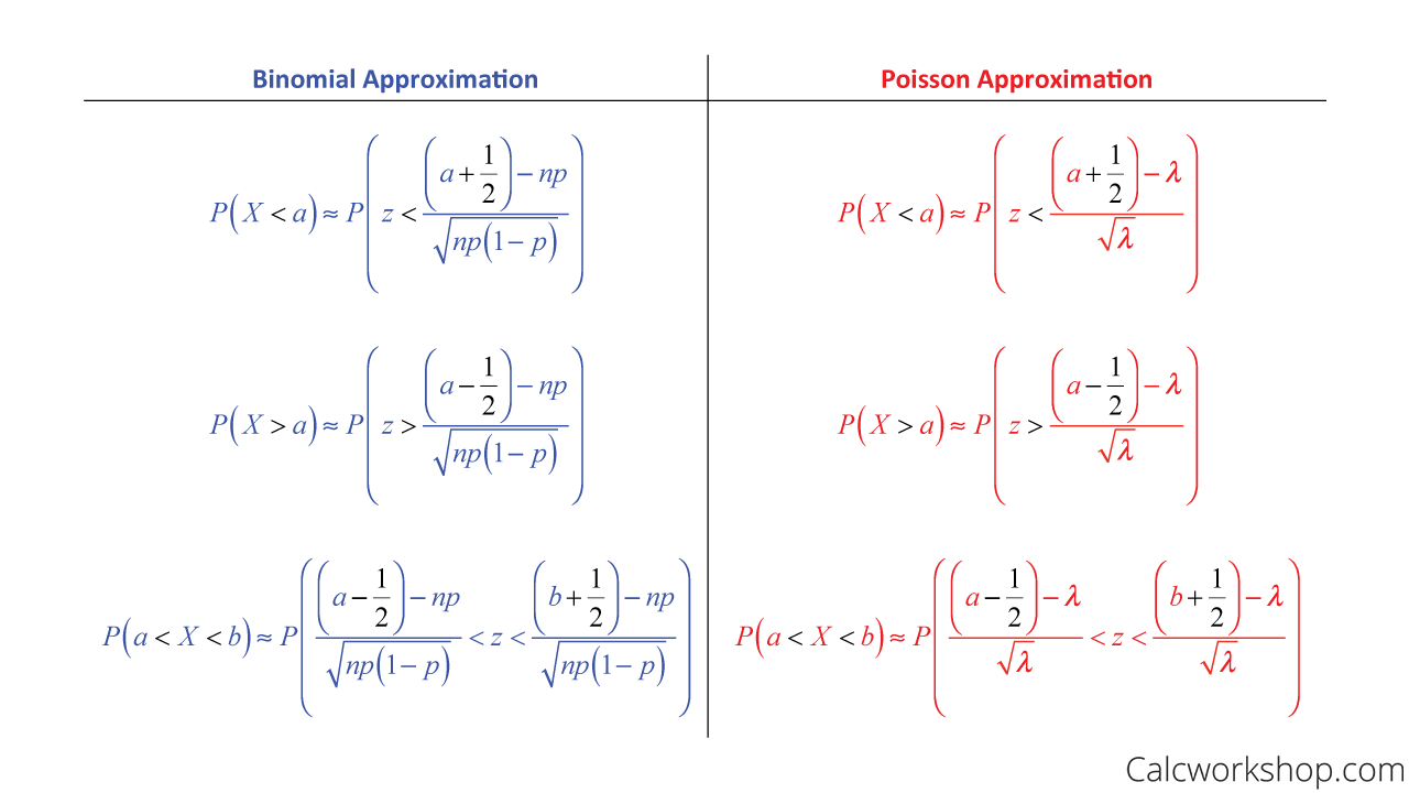
By using the following formulas!

Also, I should point out that because we are “approximating” a normal curve, we choose our x-value a little below or a little above our given value. For example, if we look at approximating the Binomial or Poisson distributions, we would say

Additionally, the Normal distribution can provide a practical approximation for the Hypergeometric probabilities too!

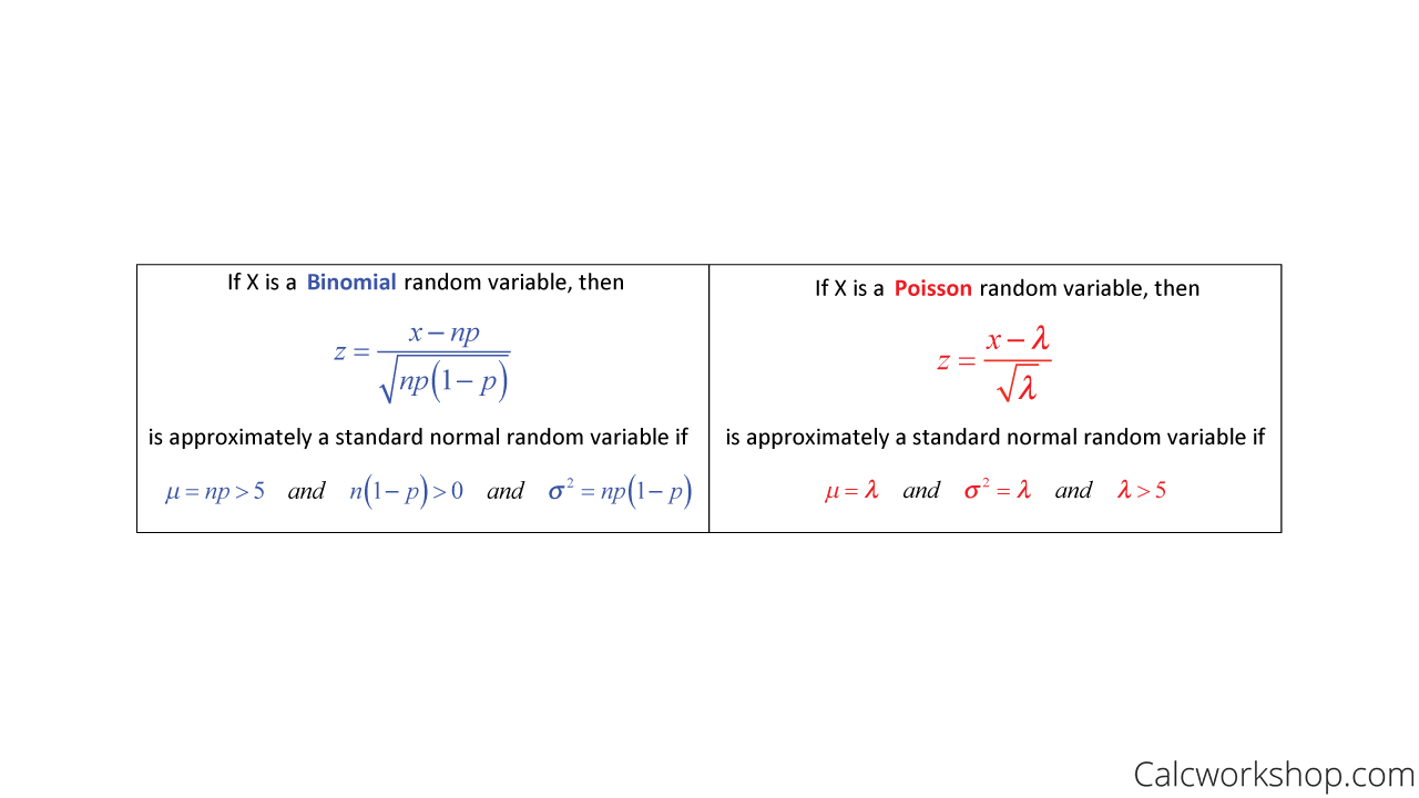
Here’s a quick look at the conditions that must be met for these discrete distributions to be approximately normal.

Example of Binomial

Okay, so now that we know the conditions and how to standardize our discrete distributions, let’s look at a few examples.

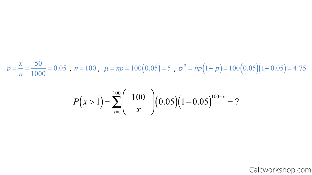
Suppose a manufacturing company specializing in semiconductor chips produces 50 defective chips out of 1,000. If 100 chips are sampled randomly, without replacement, approximate the probability that at least 1 of the chips is flawed in the sample.

First, we notice that this is a binomial distribution, and we are told that.

This would not be a very pleasant calculation to conduct. Thankfully, we are told to approximate, and that’s exactly what we’re going to do because our sample size is sufficiently large!

So, using the Normal approximation, we get

Meaning, there is a probability of 0.9805 that at least one chip is defective in the sample.

Example of Poisson

Now let’s suppose the manufacturing company specializing in semiconductor chips follows a Poisson distribution with a mean production of 10,000 chips per day. Approximate the expected number of days in a year that the company produces more than 10,200 chips in a day.

This means that if the probability of producing 10,200 chips is 0.023, we would expect this to happen approximately 365(0.023) = 8.395 days per year.

So, by the power of the Central Limit Theorem and the Law of Large Numbers, we can approximate non-normal distributions using the Standard Normal distribution where the mean becomes zero with a standard deviation of one!

This video will look at countless examples of using the Normal distribution and use it as an approximation to the Binomial distribution and the Poisson distribution.

Let’s jump on in!

Normal Approximation – Lesson & Examples (Video)

47 min

• Introduction to Video: Normal Approximation of the Binomial and Poisson Distributions
• 00:00:34 – How to use the normal distribution as an approximation for the binomial or poisson with Example #1
• Exclusive Content for Members Only

• 00:13:57 – Approximate the poisson and binomial random variables using the normal distribution(Examples #2-3)
• 00:25:41 – Find the probability of a binomial distribution using a normal approximation (Example #4)
• 00:39:40 – Find the probability of a Poisson distribution using a normal approximation (Example #5)
• Practice Problems with Step-by-Step Solutions
• Chapter Tests with Video Solutions